Basic hypothesis testing: t and F tests
Contents
Basic hypothesis testing: \(t\) and \(F\) tests
Introduction
Aims of this chapter:
Using \(t\) tests to look at differences between means
Using \(F\) tests to compare the variance of two samples
Using non-parametric tests for differences
\(t\) tests
The \(t\) test is used to compare the mean of a sample to another value, which can be:
Some reference point (Is the mean different from 5?)
Another mean (Does the mean of A differ from the mean of B?).
If you have a factor with two levels then a \(t\) test is a good way to compare the means of those samples. If you have more than two levels, then you have a problem: as the number of levels (\(n\)) increases, the number of possible comparisons between pairs of levels (\(p\)) increases very rapidly. The number of possible pairs is the binomial coefficient \(C(n,2)\) — inevitably, R has a function for this (try it in R):
choose(2:6,2)
- 1
- 3
- 6
- 10
- 15
Making these many comparisons using something like a t-test is a problem because we neglect the covariance among measures and inflate the chance of falsely rejecting at least one null hypothesis (false positive, or Type I error).
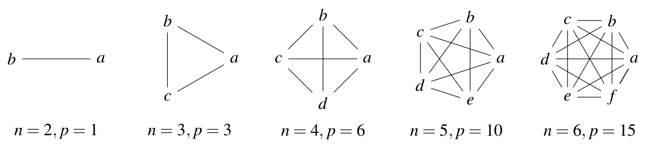
Fig. 22 Your Type I error rate increases with the number of pairwise comparisons (\(p\)) you make using a single dataset. Say, you make multiple comparisons using an \(\alpha = 0.05\) significance level. Then you have that much chance of making a Type I error on each comparison. Thus, assuming each pairwise comparison is made independently, the type I error rate just adds up with every new comparison you make. Thus, the chance of committing at least one Type I error for a set of \(n\) comparisons is \(n \times 0.05\); so for 6 pairwise comparisons, your chance of making at least one Type I (false positive) error would be \(6 \times 0.05 = 0.3\), or \(30\%\)!
A more-than-two-factors example would be if you were, say, comparing the means of more than two types of insect groups – below, we compared means of two groups (dragonflies and damselflies); if we added stoneflies to this comparison, the t-test would not be the way to go as we would be making three pairwise comparisons (n = 3, p = 3).
OK, assuming you are interested in making just one paiwise comparison, let’s learn about \(t\) tests.
The basic idea behind the \(t\) test is to divide the difference between two values by a measure of how much uncertainty there is about the size of that difference. The measure of uncertainty used is the standard error.
When there is no difference between the values \(t\) will be zero, but with big differences and/or small errors, will be larger. The \(t\) distribution below shows how commonly different values of \(t\) are found under the null hypothesis:
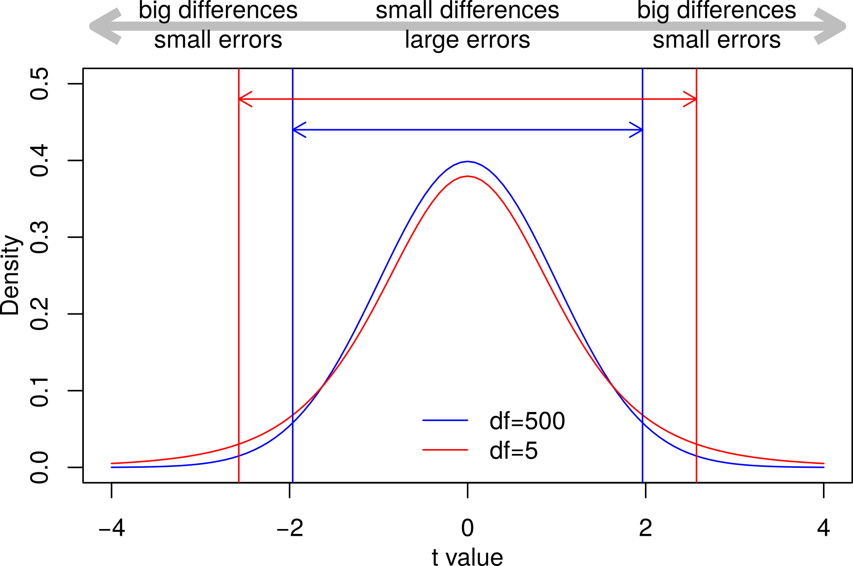
Fig. 23 The \(t\) distribution.
Some points about the \(t\)-distribution illustrated in Fig. 23:
The null hypothesis is that there is no difference between the values but because we only estimate the values from samples, differences will creep in by chance.
Mostly these differences will be small — hence the peak in the middle — but sometimes the differences will be large and the errors will be small.
95% of the area under the curves are between these two sets of vertical lines. Values of \(t\) more extreme than this will only occur 1 in 20 times or with a probability (\(p\)) of 0.05.
The means of small samples are more easily influenced by extreme values and so produce extreme \(t\) values more frequently. This is why the red curve above for smaller samples is more flattened out and why the 95% limits are more spread out.
One-sample \(t\) tests
In the simplest example, a \(t\) test can be used to test whether the mean of a sample is different from a specific value. For example:
Is the ozone in a set of air samples above the legal limit?
Is the change in a set of patients’ weights different from zero?
Is the mean genome size for Odonata smaller than 1.25 pg, which is the average for insects see here?
Oh look! We can test that last one…
Previously, we looked at the genome size and morphology of species of dragonflies and damselflies (Odonates: Anisoptera and Zygoptera). Box and whisker plots and density plots both show that the two groups have rather different genome size and morphology. We can use \(t\) tests to test whether the means of the variables of the two groups are different and we can use the \(F\) test to check whether they have the same variance.
In this chapter, we will continue to practise building scripts and creating your own R code, so we will start from an empty script file (you can refer to t_F_tests.R from TheMulQuaBio). Use this script to store the code you run in this practical session and add notes to keep a record of what each bit is doing:
\(\star\) Open R and change (setwd) to the code directory. If you have misplaced the data, download it again from TheMulQuaBio.
\(\star\) Create a new blank script called ttests.R and save it to the working directory.
\(\star\) Put a comment at the top (using #) to describe the script.
For the rest of this session, type your code into this script, adding comments and then run them in R using Ctrl+R. If you make mistakes, correct the script and run the code again. This way you will end up with a complete neat version of the commands for your analysis.
Add code to your ttests.R script to load the genome size data into R, assigning the object name genome and use str(genome) to check it has loaded correctly:
genome <- read.csv('../data/GenomeSize.csv')
To calculate a \(t\) value in a one-sample scenario, we need that observed difference and then the standard error of the difference between the mean of our sample and the known value. This is calculated using the variance and the sample size (\(n\)) of the sample (\(s\)).
This simple equation trades off variance — high variance in the data gives higher uncertainty about the location of the mean — and sample size – more data gives more certainty. So, low variance and large datasets have small standard errors; high variance and small datasets have large standard errors. Variance is calculated using sums of squares and so the square root is needed to give a standard error in the same units as the mean.
So, all we need are three values calculated from the data: mean, variance and the number of data points and we can calculate \(t\). R can do this for us.
First calculate the three values from the data:
mean.gs <- mean(genome$GenomeSize)
print(mean.gs)
[1] 1.0143
var.gs <- var(genome$GenomeSize)
    print(var.gs)
[1] 0.1396975
n.gs <- length(genome$GenomeSize)
print(n.gs)
[1] 100
Now get the difference in means:
diff <- mean.gs - 1.25
print(diff)
[1] -0.2357
Get the standard error:
se.gs <- sqrt(var.gs/n.gs)
print(se.gs)
[1] 0.03737613
Finally, get the t value
t.gs <- diff/se.gs
print(t.gs)
[1] -6.306164
This is a big \(t\) value — values this extreme don’t even appear on the graph above — so we would conclude that the mean genome size for Odonata is different from the average for insects.
\(\star\) Copy and paste the code above into your script in R and run it. Read through the code and make sure you understand the steps.
We can do the above more easily and get some more information using R’s t.test function. The null hypothesis can be set using the option (sometimes called a function argument) mu — the Greek letter \(\mu\) is typically used to refer to a (true, not sample) mean:
t.test(genome$GenomeSize, mu = 1.25)
	One Sample t-test

data:  genome$GenomeSize
t = -6.3062, df = 99, p-value = 8.034e-09
alternative hypothesis: true mean is not equal to 1.25
95 percent confidence interval:
 0.9401377 1.0884623
sample estimates:
mean of x
   1.0143
This confirms the values we calculated by hand and adds a \(p\) value. The output also gives the degrees of freedom. This is something we will come back to later, but the degrees of freedom are basically the number of data points minus the number of estimated parameters, which in this case is one mean.
Confidence Intervals
The output also gives a confidence interval for the observed mean. The mean is the best estimate of the population mean given our sample of species of Odonata, but the actual mean for the order could be bigger or smaller. The confidence interval tells us the region in which we are 95% confident that this actual mean lies.
It is calculated using the \(t\) distribution. Remember that \(t\) is a difference divided by a standard error; if we multiply \(t\) by a standard error, we get back to a difference. If we pick a pair of \(t\) values that contain the middle 95% of the \(t\) distribution, as in the plot on page 2, then we can multiply that by the standard error from the data to get a range above and below the mean. If we sampled lots of sets of 100 species of Odonata, we expect 95% of the observed means to lie inside this range. The code below shows the calculation of the confidence interval for the test above.
First, find the edges of the middle 95% of a \(t\) distribution with 99 df:
tlim <- qt(c(0.025,0.975), df = 99)
print(tlim)
[1] -1.984217 1.984217
(quantiles of the t distribution, so qt)
Now use the mean and standard error from above to get a confidence intervals:
mean.gs + tlim * se.gs
- 0.940137655780312
- 1.08846234421969
Exercise
Using the t.test code above as a template, test whether the body weight (in grams) of Odonata is different from the average for arthropods of 0.045 grams. Note that this slightly dodgy estimate comes from an estimated average volume for arthropods of 45.21 mm\(^3\), and assuming a density of 1 gm per cm\(^3\); see:
Orme, C. D. L., Quicke, D. L. J., Cook, J. M. and Purvis, A. (2002), Body size does not predict species richness among the metazoan phyla. Journal of Evolutionary Biology, 15: 235–247.
Two-sample \(t\) tests
It is more common to use a \(t\) test to compare the means of two samples. This includes questions like:
Do two rivers have the same concentration of a pollutant?
Do chemicals A and chemical B cause different rates of mutation?
Do damselflies and dragonflies have different genome sizes?
The main difference here is that with a one sample \(t\) test, we assume that one of the means is known exactly: the only error is in the single sample. With a two sample test, we are comparing two means estimated from samples and both contain error. The graph below illustrates this:
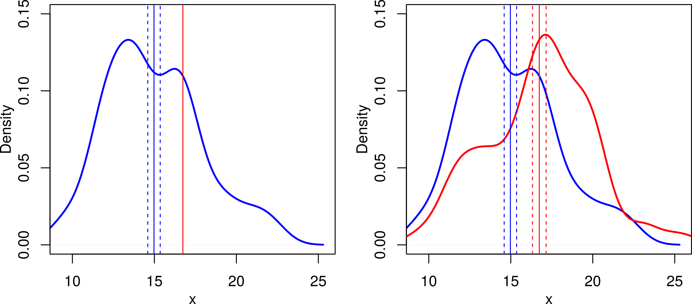
Fig. 24 Illustration of one-sample (left) vs. two-sample (right) \(t\) tests. The vertical lines show the mean (solid lines) and one standard error to each side (dashed lines). The red mean is the same in both cases, but the second graph shows that this is also estimated from a sample with error: the difference in the means looks less convincing and we’d expect a smaller \(t\) value.
A few points to note about Fig. 24:
The \(t\) tests in for these two graphs confirm this:
The mean for blue is significantly different from 16.74 (mean=14.98, se=0.38, df=59, \(t\)=-4.65, \(p\)=0.00002).
The means of blue and red are significantly different (blue: mean=14.98, se=0.38; red: mean=16.74, se=0.42; df=118, \(t\)=-3.13, \(p\)=0.002)
\(\star\) Have a close look at the previous two statements. This shows the kind of detail needed when reporting the results of \(t\) tests. The following is not acceptable: The means of blue and red are significantly different (\(p=0.002\)).
So, with two samples, we shouldn’t be so confident about the difference between the values — it should have a higher standard error. We can do this simply by combining the variance and sample size for the two samples (\(a\) and \(b\)) into the calculation:
Note that the two-sample t-test makes two assumptions; that the data are:
(i) normally distributed, so that the two means are a good measure of central tendencies of the two samples and be estimated sensibly; and
(ii) have similar variances.
The first assumption also applies to the one-sample t-test.
Let’s use a \(t\) test to address the question of whether the genome sizes of Anisoptera and Zygoptera are different. First, we’ll do this by hand.
We’ll use a really handy function tapply(X, INDEX, FUN) to quickly find the values for the two groups: it takes some values (X), splits those values into groups based on a factor (INDEX) and runs each group through another function (FUN).
So let’s first calculate the three values from the data:
mean.gs <- tapply(X = genome$GenomeSize, INDEX = genome$Suborder, FUN = mean)
print(mean.gs)
Anisoptera  Zygoptera
  1.011774   1.018421
var.gs <- tapply(X = genome$GenomeSize, INDEX = genome$Suborder, FUN = var)
print(var.gs)
Anisoptera  Zygoptera
 0.1845755  0.0694569
n.gs <- tapply(X = genome$GenomeSize, INDEX = genome$Suborder, FUN = length)
print(n.gs)
Anisoptera  Zygoptera
        62         38
Now get the difference in means:
diff <- mean.gs[1] - mean.gs[2]
print(diff)
  Anisoptera
-0.006646859
Now get the standard error of the difference:
se.gs <- sqrt((var.gs[1]/n.gs[1]) + (var.gs[2]/n.gs[2]))
print(se.gs)
Anisoptera
0.06931693
And finally, the t-value.
t.gs <- diff/se.gs
print(t.gs)
 Anisoptera
-0.09589084
\(\star\) Type the above code into your growing R script and run it in R. Again, read through the code and make sure you understand the steps.
And as before, the t.test function can be used to automate this all for us. We can use a formula as we have seen before to get a test between the two suborders:
t.test(GenomeSize ~ Suborder, data = genome)
	Welch Two Sample t-test

data:  GenomeSize by Suborder
t = -0.095891, df = 97.997, p-value = 0.9238
alternative hypothesis: true difference in means is not equal to 0
95 percent confidence interval:
 -0.1442041  0.1309104
sample estimates:
mean in group Anisoptera  mean in group Zygoptera
                1.011774                 1.018421
The output looks very similar to the one-sample t-test, except that the output now gives two estimated means, rather than one and it reports the \(p\) value for the calculated \(t\) value.
Confidence Intervals again
Also, in the output above unlike the 95% interval of a 1 sample t-test, which provides the confidence intervals around the estimated mean of the single population, this output of the 2-sample test provides the confidence intervals around the observed difference in the means of the two samples. That is, the 95% confidence interval (-0.1442041, 0.1309104) above is around the observed difference in the sample means: \(1.011774 - 1.018421 = - 0.006647\). This is essentially not distinguishable from zero as the intervals include the value 0 (and therefore, the p-value is also insignificant).
\(\star\) Add this last step to your script and run it.
Exercise
\(\star\) Expand your t-test code to test whether the body weight of the two suborders are different and add it to in the script file.
The \(F\) test
The \(F\) test is used to compare the variances of two samples or populations. You will also see them featured in analysis of variance (ANOVA), to test the hypothesis that the means of a given set of normally distributed populations all have the same variance.
The distribution of the test statistic \(F\) (the \(F\) distribution) is simply the ratio of the variances for sample \(a\) and \(b\): \(\frac{\textrm{var}(a)}{\textrm{var}(b)}\):
If the two variances are the same then \(F=1\);
if \(\textrm{var}(a) > \textrm{var}(b)\) then \(F > 1\);
and if \(\textrm{var}(a) < \textrm{var}(b)\) then \(F < 1\)
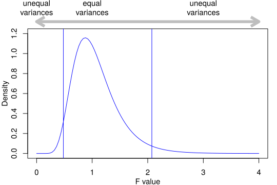
Fig. 25 The F distribution. The two vertical blue lines show the edges of the central 95% of the area of the curve.
In the above figure, note that:
If the two samples are drawn at random from a population with the same variance then values of \(F < 0.482\) or \(> 2.074\) are observed fewer than 1 time in 20 (\(p \le 0.05\) ). And because \(1/0.482 \approx 2.074\) and \(1/2.074 \approx 0.482\), in this case, it doesn’t matter which way round you compare the two variances. This is not always true, and the order in which you compare two variances will very often matter.
The shape of the \(F\) distribution changes depending on the amount of data in each of the two samples but will always be centered near 1 and with a tail to the right (right-skewed).
This F-distribution arises as the ratio of two appropriately scaled chi-square distributed variates, because, as we saw above, variances should be chi-square distributed.
Let’s use our same genome size dataset to learn how to do F-tests as well. We will use the F test to judge whether a key assumption of the two-sample \(t\) tests we did above holds: that the two samples have equal variances.
First, let’s visualize the data. As I hope you’ve already noticed, this session has been neglecting one very important part of analysis — plotting the data.
We are going to compare two plots, so it helps to have them side by side in the same window. We can use the function par to change a set of options called graphics parameters to get R to do this. The option to change is mfrow. This sets a graphics window to include multiple figures and we need to tell R the number of rows and columns to divide the window into: par(mfrow=c(1,2)).
\(\star\) Type par(mfrow=c(1,2)) into your script, add a comment, and run it.
Using your (rapidly improving!) R skills, create a boxplot comparing the genome sizes of the two suborders.
Add another boxplot beside it comparing the body weight of the two suborders.
It should look like Fig. 26.

Fig. 26 Reproduce this figure.
Now, we can use R to calculate \(F\) for the variance in genome size in each of the two suborders. We calculated the variance for the \(t\) test above, so we can just do this:
var.gs[1]/var.gs[2]
That’s quite a big \(F\) value and we can use the function var.test to do all the calculations for us and give us the actual \(p\) value:
var.test(GenomeSize ~ Suborder, data = genome)
	F test to compare two variances

data:  GenomeSize by Suborder
F = 2.6574, num df = 61, denom df = 37, p-value = 0.001946
alternative hypothesis: true ratio of variances is not equal to 1
95 percent confidence interval:
 1.449330 4.670705
sample estimates:
ratio of variances
           2.65741
It produces the same value that we calculated by hand and shows that, if the two samples are drawn from populations with the same variance, an \(F\) value this extreme will only be observed roughly 1 time in 500 (\(1/0.00195 \approx 500\)) .
\(\star\) Open a new empty script called FTests.R.
In this write your script to test whether the variances in the body weight of the two suborders from the GenomSize dataset are different.
There are clearly problems with the variance in both examples. The next two sections present ways to address these kinds of problems.
\(t\) tests revisited
The first thing to say is that R is aware of the problem with the variance. If you look back at the output from the previous \(t\) tests, you will see that the degrees of freedom vary a lot. We have 100 observations and – after subtracting one for each mean we calculate — our degrees of freedom should be either 99 (one sample test) or 98 (two
sample test). What we actually see are smaller numbers, with the smallest being df = 60.503 for the two sample test of body weight.
The explanation is that R is applying a penalty to the degrees of freedom to account for differences in variance. With fewer degrees for freedom, more extreme \(t\) values are more likely and so it is harder to find significant results. This doesn’t mean we can forget about checking the variances or plotting the data!
In this case, we can also apply a transformation to the data in order to make the variances more equal. Forgetting the wings and assuming Odonata are shaped like a box, the model in the graph below shows how volume changes with length: equal changes in length do not lead to equal changes in volume and longer species will have a disproportionately large volume. This is a classic feature of morphological data known as allometric scaling and we’ll look at it again when we learn about ANOVA.
In the meantime, a log transformation will turn body weight from a skewed distribution to a more normal distribution, as shown in Fig. 27.
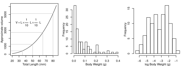
Fig. 27 Log transformation of body weights.
We can do a \(\log_e\) (natural log) transform of our body weight data as follows:
genome$logBodyWeight <- log(genome$BodyWeight)
That is, you took a natural log of the whole Body weight column and saved it as a new column called logBodyWeight
\(\star\) Copy the line into your FTests.R script and run it.
Exercise
Now write three lines of code to get a boxplot of \(\log_e\) body weight and then run a variance test and \(t\) test on the differences in \(\log_e\) body weight between suborders. This gives a much clearer result — the variances are almost identical and the differences between the suborders are much more cleanly tested.
Non-parametric tests
What happens if there isn’t a convenient transformation for the variable that gives roughly constant variation and equal variance? In a parametric test, like the \(t\) and \(F\) test above, we use parameters (mean and variance) to describe the data, assume these describe the data well and then just use these parameters to run the test. If these assumptions don’t seem very sound, the non-parametric tests provide a way of using the ranks of the data to test for differences. They aren’t as powerful — they are less likely to reveal significant differences — but they are more robust. The most commonly used alternative is the Wilcoxon test, which uses the function wilcox.test in R.
\(\star\) Using wilcox.test as a replacement for t.test, repeat the one and two sample \(t\) test for genome size and body weight.
For example to carry out a wilcox test equivalent to the one-sample t test you performed above:
wilcox.test(genome$GenomeSize, mu=1.25)
	Wilcoxon signed rank test with continuity correction

data:  genome$GenomeSize
V = 893.5, p-value = 2.043e-08
alternative hypothesis: true location is not equal to 1.25
Compare the two (t vs wilcox test) results.
Exercise
Repeat the above analyses with the predator and prey body mass data that you were introduced to previously. Again check how different the results are when using \(t\) vs. Wilcoxon tests.