Biological Computing in R¶

Introduction¶

R is a freely available statistical software with strong programming capabilities widely used by professional scientists around the world. It was based on the commercial statistical software S by Robert Gentleman and Ross Ihaka. The first stable version appeared in 2000. It was essentially designed for programming statistical analysis and data-mining. It became the standard tool for data analysis and visualization in biology in a matter of just 10 years or so. It is also frequently used for mathematical modelling in biology.

This chapter aims to lay down the foundations for you to use R for scientific computing in biology by exploiting it full potential as a fully featured object-oriented programming language. Specifically, this chapter aims at teaching you:

Basic R syntax and programming conventions, assuming you have never set your eyes on R
Principles of data processing and exploration (including visualization) using R
Principles of clean and efficient programming using R
To generate publication quality graphics in R
To develop reproducible data analysis “work flows” so you (or anybody else) can run and re-run your analyses, graphics outputs and all, in R
To make R simulations more efficient using vectorization
To find and fix errors in R code using debugging
To make data wrangling and analyses more efficient and convenient using special packages
Some additional, advanced topics (accessing databases, building your own packages, etc.).

Why R?¶

There are many commercial statistical (minitab, SPSS, etc) software packages in the world that are mouse-driven, warm, and friendly, and have lots of statistical tests and plotting/graphing capabilities. Why not just use them? Here are some very good reasons:

R has numerous tried and tested packages for data-handling and processing
R provides basically every statistical test you’ll ever need and is constantly being improved. You can tailor your analyses rather than trying to use the more limited options each statistical software package can offer.
R has excellent graphing and visualization capabilities and produce publication-quality graphics that can be re-produced with scripts – you won’t get RSI mouse-clicking your way though graphing and re-graphing your data every time you change your analysis!
It also has good capabilities for mathematical calculations, including matrix algebra
R is scriptable, so you can build a perfectly repeatable record of your analysis. This in itself has several advantages:
- You can never replicate exactly the same analysis with all the same steps using a point-and-click approach/software. With R you can reproduce your full analysis for yourself (in the future!), your colleagues, your supervisor/employer, and any journal you might want to submit your work to.
- You may need to rerun your analysis every time you get new data. Once you have it all in a R script, you can just rerun your analysis and go home!
- You may need to tweak your analysis many times (new data, supervisor changes mind, you change mind, paper reviewers want you do something differently). Having the analysis recorded as script then allows you to do so by revising the relevant parts of your analysis with relatively little pain.
R is freely available for all common computer operating systems – if you want a copy on your laptop, help yourself at the CRAN website.
Being able to program in R means you can develop and automate your own data handling, statistical analysis, and graphing/plotting, a set of skills you are likely to need in many, if not most careers paths.

Would you ever need anything other than R?¶

Being able to program R means you can develop and automate your statistical analyses and the generation of figures into a reproducible work flow. For many of you, using R as your only programming language will do the job. However, if your work also includes extensive numerical simulations, manipulation of very large matrices, bioinformatics, relational database access and manipulation, or web development, you will be better-off also knowing another programming language that is more versatile and computationally efficient (like Python or Julia).

Installing R¶

If you are using a college computer, R will likely already be available.

Otherwise you can follow these instructions to install R on your own computer.

In particular, on Ubuntu Linux, it is as simple as typing the following in terminal:

sudo apt install r-base r-base-dev

Getting started¶

You should be using an IDE for R. Please re-visit the “To IDE or not to IDE” section of the Introduction if you are not familiar with IDEs.

Let’s briefly look at the bare-bones R interface and command line interface (CLI), and then switch to an IDE like Visual Studio Code or RStudio.

Launch R (From Applications menu on Window or Mac, from terminal in Linux/Ubuntu) — it should look something like this (on Linux/Ubuntu or Mac terminal):

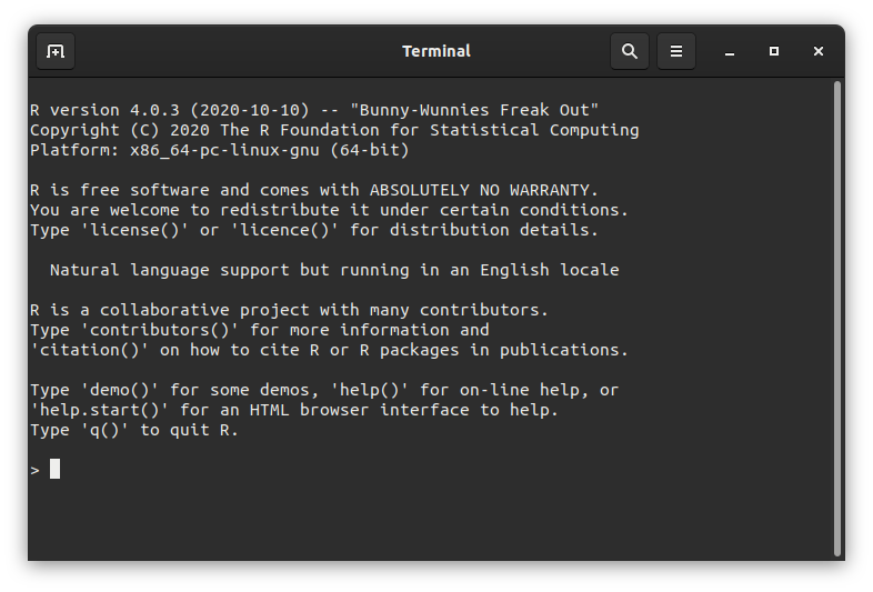
Fig. 14 The R console in Linux/Unix.¶

Or like this (Windows “console”, similar in Mac):

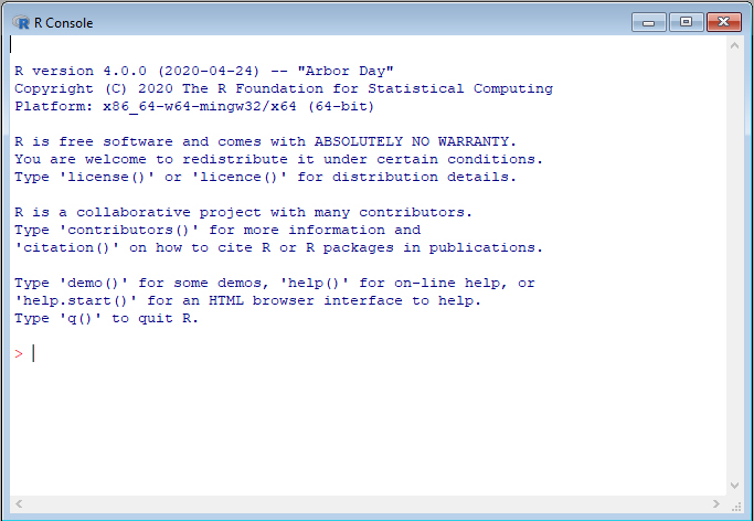
Fig. 15 The R console in Windows/Mac OS.¶

R basics¶

Lets get started with some R basics. You will be working by entering R commands interactively at the R user prompt (>). Up and down arrow keys scroll through your command history.

Useful R commands¶

Command	What it does
`ls()`	list all the variables in the work space
`rm('a', 'b')`	remove variable(s) `a` and `b`
`rm(list=ls())`	remove all variable(s)
`getwd()`	get current working directory
`setwd('Path')`	set working directory to `Path`
`q()`	quit R
`?Command`	show the documentation of `Command`
`??Keyword`	search the all packages/functions with ‘Keyword’, “fuzzy search”

Baby steps¶

Like in any programming language, you will need to use “variables” to store information in a R session’s workspace. Each variable has a reserved location in your RAM, and takes up “real estate” in it — that is when you create a variable you reserve some space in your computer’s memory.

★ Now, let’s try assigning a few variables in R and doing things to them:

a <- 4  # store 4 as variable a

a # display it

4

a * a # product

16

Store a variable:

a_squared <- a * a 

Note

Unlike Python or most other programming languages, R uses the <- operator to assign variables. You can use = as well, but it does not work everywhere, so better to stick with <-.

sqrt(a_squared) # square root

4

Build a vector with c (stands for “concatenate”):

v <- c(0, 1, 2, 3, 4)

v # Display the vector-valued variable you created

0
1
2
3
4

Note that any text after a “#” is ignored by R, like in many other languages — handy for commenting.

*In general, please comment your code and scripts, for everybody’s sake. You will be amazed by how difficult it is to read and understand what a certain R script does (or any other script, for that matter) without judicious comments — even scripts you yourself wrote not so long ago!

Tip

The Concatenate function: c()(concatenate) is one of the most commonly used R functions because it is the default method for combining multiple arguments into a vector. To learn more about it, type ?c at the R prompt and hit enter.

is.vector(v) # check if v's a vector

TRUE

mean(v) # mean

2

Thus, a vector is like a single column or row in a spreadsheet (just like it is in Python). Multiple vectors can be combined to make a matrix (the full spreadsheet).

This is one of many ways R stores and processes data. More on R data types and objects below.

A single value (any kind) is a vector object of length 1 by default. That’s why in the R console you see [1] before any single-value output (e.g., type 8, and you will see [1] 8).

Some examples of operations on vectors:

var(v) # variance

2.5

median(v) # median

2

sum(v) # sum all elements

10

prod(v + 1) # multiply

120

length(v) # how many elements in the vector

5

Variable names and Tabbing¶

In R, you can name variables in the following way to keep track of related variables:

wing.width.cm <- 1.2 #Using dot notation

wing.length.cm <- c(4.7, 5.2, 4.8)

This can be handy; type:

wing.

And then hit the tabkey to reveal all variables in that category. This is nice — variable names should be as obvious as possible. However, they should not be over-long either! Good style and readability is more important than just convenient variable names.

In fact, R allows dots to be used in variable names of all objects (not just objects that are variables). For example, functions names can have dots in them as well, as you will see below with the is.* family (e.g., is.infinite(), is.nan(), etc.).

Tip

Following a consistent style for different elements of your R code (synttax, conditionals, functions, etc) is important. The tidyverse style guide is recommended. While should keep going back to difefrent sections of the syule gude as you learn new topics. Here, for starters, have a look at naming conventions.

Operators¶

The usual operators are available in R:

Operator
`+`	Addition
`-`	Subtraction
`*`	Multiplication
`/`	Division
`^`	Power
`%%`	Modulo
`%/%`	Integer division
`==`	Equals
`!=`	Differs
`>`	Greater
`>=`	Greater or equal
`&`	Logical and
`	`
`!`	Logical not

When things go wrong¶

Here are some common syntax errors that you might run into in R, especially when you just beginning to learn this language:

Missing a closing bracket leads to continuation line, which looks something like this, with a + at the end:

x <- (1 + (2 * 3)
+ 

Hit Ctrl-C(UNIX terminal or base R command line) or ESC (in in RStudio) or keep typing!

Too many parentheses; for example, 2 + (2*3))
Wrong or mismatched brackets (see next subsection)
Mixing double and single quotes will also give you an error

When things are taking too long and the R console seems frozen, try Ctrl + C (UNIX terminal or base R command line) or ESC (in RStudio) to force an exit from whatever is going on.

Types of parentheses¶

R has specific uses for different types of Parentheses type that you need to get used to:

Parentheses type	What it does
`f(3,4)`	call the function (or command) f, with the arguments 3 & 4.
`a + (b*c)`	to enforce order over which statements or calculations are executed. Here `(bc)`is executed before adding to `a`. Here is an alternative order: `(a + b)c`
`{expr1; expr2;...exprn}`	group a set of expressions or commands into one compound expression. Value returned is value of last expression; used in building function, loops, and conditionals (more on these soon!).
`x[4]`	get the 4th element of the vector `x`.
`li[[3]]`	get the 3rd element of some list `li`, and return it.(compare with `li[3]`, which returns a list with just the 3rd element inside). More on lists in next section.

li = list(c(1,2,3))

class(li)

'list'

Variable types¶

There are different kinds of data variable types in R, but you will basically need to know four for most of your work: integer, float (or “numeric”, including real numbers), string (or “character”, e.g., text), and Boolean (“logical”; Trueor FALSE).

Try this:

v <- TRUE

TRUE

class(v)

'logical'

The class() function tells you what type of variable any object in the workspace is.

v <- 3.2
class(v)

'numeric'

v <- 2L
class(v)

'integer'

v <- "A string"
class(v)

'character'

b <- NA
class(b)

'logical'

Also, the is.* family of functions allow you to check if a variable is a specific in R:

is.na(b)

TRUE

b <- 0/0
b

NaN

is.nan(b)

TRUE

b <- 5/0
b

Inf

is.nan(b)

FALSE

Tip

Beware of the difference between NA (Not Available) and NaN (Not a Number). R will use NAto represent/identify missing values in data or outputs, while NaNrepresent nonsense values (e.g., 0/0) that cannot be represented as a number or some other data type.

See what R has to say about this: try ?is.nan, ?is.na, ?NA, ?NaNin the R commandline (one at a time!).

There are also Inf (Infinity, e.g., 1/0), and NULL (variable not set) value types. Look these up as well using ?.

is.infinite(b)

TRUE

is.finite(b)

FALSE

is.finite(0/0)

FALSE

Type Conversions and Special Values¶

The as.* commands all convert a variable from one type to another. Try out the following examples:

as.integer(3.1)

3

as.numeric(4)

4

as.roman(155)

[1] CLV

as.character(155)  # same as converting to string

'155'

as.logical(5)

TRUE

What just happened?! R maps all values other than 0 to logical True, and 0 to False. This can be useful in some cases, for example, when you want to convert all your data to Presence-Absence only.

as.logical(0)

FALSE

Also, keep an eye out for E notation in outputs of R functions for statistical analyses, and learn to interpret numbers formatted this way. R uses E notation in outputs of statistical tests to display very large or small numbers. If you are not used to different representations of long numbers, the E notation might be confusing.

Try this:

1E4

10000

1e4

10000

5e-2

0.05

1E4^2

1e+08

1 / 3 / 1e8

3.33333333333333e-09

Tip

Boolean arguments in R: In R, you can use F and T for boolean FALSE and TRUE respectively. To see this, type

a <- T

in the R commandline, and then see what R returns when you type a. Using F and T for boolean FALSE and TRUE respectively is not necessarily good practice, but be aware that this option exists.

R Data Structures¶

R comes with different built-in structures (objects) for data storage and manipulation. Mastering these, and knowing which one to use when will help you write better, more efficient programs and also handle diverse datasets (numbers, counts, names, dates, etc).

Note

Data “structures” vs. “objects” in R: You will often see the terms “object” and “data structure” used in this and other chapters. These two have a very distinct meaning in object-oriented programming (OOP) languages like R and Python. A data structure is just a “dumb” container for data (e.g., a vector). An object, on the other hand can be a data structure, but also any other variable or a function in your R environment. R, being an OOP language, converts everything in the current environment to an object so that it knows what to do with each such entity — each object type has its own set of rules for operations and manipulations that R uses when interpreting your commands.

Vectors¶

The Vector, which you have already seen above, is a fundamental data object / structure in R. Scalars (single data values) are treated as vector of length 1. A vector is like a single column or row in a spreadsheet.

★ Now get back into R (if you somehow quit R using q()or something else), and try this:

a <- 5
is.vector(a)

TRUE

v1 <- c(0.02, 0.5, 1)
v2 <- c("a", "bc", "def", "ghij")
v3 <- c(TRUE, TRUE, FALSE)

v1;v2;v3

0.02
0.5
1

'a'
'bc'
'def'
'ghij'

TRUE
TRUE
FALSE

R vectors can only store data of a single type (e.g., all numeric or all character). If you try to combine different types, R will homogenize everything to the same data type. To see this, try the following:

v1 <- c(0.02, TRUE, 1)
v1

0.02
1
1

TRUE gets converted to 1.00!

v1 <- c(0.02, "Mary", 1)
v1

'0.02'
'Mary'
'1'

Everything gets converted to text!

Basically, the function c “coerces” arguments that are of mixed types (strings/text, real numbers, logical arguments, etc) to a common type.

Matrices and arrays¶

A R “matrix” is a 2 dimensional vector (has both rows and columns) and a “array” can store data in more than two dimensions (e.g., a stack of 2-D matrices).

R has many functions to build and manipulate matrices and arrays.

Try this:

mat1 <- matrix(1:25, 5, 5)
mat1

A matrix: 5 × 5 of type int
1	6	11	16	21
2	7	12	17	22
3	8	13	18	23
4	9	14	19	24
5	10	15	20	25

Note that the output in your terminal or console will be more like:

print(mat1)

     [,1] [,2] [,3] [,4] [,5]
[1,]    1    6   11   16   21
[2,]    2    7   12   17   22
[3,]    3    8   13   18   23
[4,]    4    9   14   19   24
[5,]    5   10   15   20   25

(even if you don’t use the print() command)

The output looks different above because the R code is running in a jupyter notebook.

Now try this:

mat1 <- matrix(1:25, 5, 5, byrow=TRUE)
mat1

A matrix: 5 × 5 of type int
1	2	3	4	5
6	7	8	9	10
11	12	13	14	15
16	17	18	19	20
21	22	23	24	25

That is, you can order the elements of a matrix by row instead of column (default).

dim(mat1) #get the size of the matrix

5
5

To make an array consisting of two 5$\times$5 matrices containing the integers 1-50:

arr1 <- array(1:50, c(5, 5, 2))
arr1[,,1]

A matrix: 5 × 5 of type int
1	6	11	16	21
2	7	12	17	22
3	8	13	18	23
4	9	14	19	24
5	10	15	20	25

print(arr1)

, , 1

     [,1] [,2] [,3] [,4] [,5]
[1,]    1    6   11   16   21
[2,]    2    7   12   17   22
[3,]    3    8   13   18   23
[4,]    4    9   14   19   24
[5,]    5   10   15   20   25

, , 2

     [,1] [,2] [,3] [,4] [,5]
[1,]   26   31   36   41   46
[2,]   27   32   37   42   47
[3,]   28   33   38   43   48
[4,]   29   34   39   44   49
[5,]   30   35   40   45   50

arr1[,,2]

A matrix: 5 × 5 of type int
26	31	36	41	46
27	32	37	42	47
28	33	38	43	48
29	34	39	44	49
30	35	40	45	50

Just like R vectors, R matrices and arrays have to be of a homogeneous type, and R will do the same sort of type homogenization you saw for R vectors above.

Try inserting a text value in mat1and see what happens:

mat1[1,1] <- "one"
mat1

A matrix: 5 × 5 of type chr
one	2	3	4	5
6	7	8	9	10
11	12	13	14	15
16	17	18	19	20
21	22	23	24	25

mat1 went from being A matrix: 5 × 5 of type int to A matrix: 5 × 5 of type chr. That is, inserting a string in one location converted all the elements of the matrix to the chr (string) data type.

Thus R’s matrix and array are similar to Python’s numpy array and matrix data structures.

Data frames¶

This is a very important data structure in R. Unlike matrices and vectors, R data frames can store data in which each column contains a different data type (e.g., numbers, strings, boolean) or even a combination of data types, just like a standard spreadsheet. Indeed, the dataframe data type was built to emulate some of the convenient properties of spreadsheets. Many statistical and plotting functions and packages in R naturally use data frames.

Let’s build and manipulate a dataframe. First create three vectors:

Note

Under the hood, a R data frame is in fact a list of equal-length vectors.

Col1 <- 1:10
Col1

1
2
3
4
5
6
7
8
9
10

Col2 <- LETTERS[1:10]
Col2

'A'
'B'
'C'
'D'
'E'
'F'
'G'
'H'
'I'
'J'

Col3 <- runif(10) # 10 random numbers from a uniform distribution
Col3

0.938413555268198
0.426268232986331
0.352635570103303
0.420346662169322
0.309041227446869
0.0709800566546619
0.294151729205623
0.802815589588135
0.706063920864835
0.974233828950673

Now combine them into a dataframe:

MyDF <- data.frame(Col1, Col2, Col3)
MyDF

A data.frame: 10 × 3
Col1	Col2	Col3
<int>	<chr>	<dbl>
1	A	0.93841356
2	B	0.42626823
3	C	0.35263557
4	D	0.42034666
5	E	0.30904123
6	F	0.07098006
7	G	0.29415173
8	H	0.80281559
9	I	0.70606392
10	J	0.97423383

Again, this output looks different from your terminal/console output because these commands are running in a Jupyter notebook.

Your output will look like this:

print(MyDF)

   Col1 Col2       Col3
   1    A 0.93841356
   2    B 0.42626823
   3    C 0.35263557
   4    D 0.42034666
   5    E 0.30904123
   6    F 0.07098006
   7    G 0.29415173
   8    H 0.80281559
   9    I 0.70606392
 10    J 0.97423383

You can easily assign names to the columns of dataframes:

names(MyDF) <- c("MyFirstColumn", "My Second Column", "My.Third.Column")
MyDF

A data.frame: 10 × 3
MyFirstColumn	My Second Column	My.Third.Column
<int>	<chr>	<dbl>
1	A	0.93841356
2	B	0.42626823
3	C	0.35263557
4	D	0.42034666
5	E	0.30904123
6	F	0.07098006
7	G	0.29415173
8	H	0.80281559
9	I	0.70606392
10	J	0.97423383

And unlike matrices, you can access the contents of data frames by naming the columns directly using a $ sign:

MyDF$MyFirstColumn

1
2
3
4
5
6
7
8
9
10

But don’t use spaces in column names! Try this:

MyDF$My Second Column

Error in parse(text = x, srcfile = src): <text>:1:9: unexpected symbol
1: MyDF$My Second
            ^
Traceback:

That gives an error, because R cannot handle spaces in column names easily.

So replace that column name using the colnames function:

colnames(MyDF)

'MyFirstColumn'
'My Second Column'
'My.Third.Column'

colnames(MyDF)[2] <- "MySecondColumn"
MyDF

A data.frame: 10 × 3
MyFirstColumn	MySecondColumn	My.Third.Column
<int>	<chr>	<dbl>
1	A	0.93841356
2	B	0.42626823
3	C	0.35263557
4	D	0.42034666
5	E	0.30904123
6	F	0.07098006
7	G	0.29415173
8	H	0.80281559
9	I	0.70606392
10	J	0.97423383

But using dots in column names is OK (just as it is for variable names):

MyDF$My.Third.Column

0.938413555268198
0.426268232986331
0.352635570103303
0.420346662169322
0.309041227446869
0.0709800566546619
0.294151729205623
0.802815589588135
0.706063920864835
0.974233828950673

You can also access elements by using numerical indexing:

MyDF[,1]

1
2
3
4
5
6
7
8
9
10

That is, you asked R to return values of MyDF in all Rows (therefore, nothing before the comma), and the first column (1 after the comma).

MyDF[1,1]

1

MyDF[c("MyFirstColumn","My.Third.Column")] # show two specific columns only

A data.frame: 10 × 2
MyFirstColumn	My.Third.Column
<int>	<dbl>
1	0.93841356
2	0.42626823
3	0.35263557
4	0.42034666
5	0.30904123
6	0.07098006
7	0.29415173
8	0.80281559
9	0.70606392
10	0.97423383

You can check whether a particular object is a dataframe data structure with:

class(MyDF)

'data.frame'

You can check the structure of a dataframe with str():

str(MyDF)

'data.frame':	10 obs. of  3 variables:
 $ MyFirstColumn  : int  1 2 3 4 5 6 7 8 9 10
 $ MySecondColumn : chr  "A" "B" "C" "D" ...
 $ My.Third.Column: num  0.938 0.426 0.353 0.42 0.309 ...

You can print the column names and top few rows with head():

head(MyDF)

A data.frame: 6 × 3
	MyFirstColumn	MySecondColumn	My.Third.Column
	<int>	<chr>	<dbl>
1	1	A	0.93841356
2	2	B	0.42626823
3	3	C	0.35263557
4	4	D	0.42034666
5	5	E	0.30904123
6	6	F	0.07098006

And the bottom few rows with tail():

tail(MyDF)

A data.frame: 6 × 3
	MyFirstColumn	MySecondColumn	My.Third.Column
	<int>	<chr>	<dbl>
5	5	E	0.30904123
6	6	F	0.07098006
7	7	G	0.29415173
8	8	H	0.80281559
9	9	I	0.70606392
10	10	J	0.97423383

Note

The Factor data type: R has a special data type called “factor”. Different values in this data type are called “levels”. This data type is used to identify “grouping variables” such as columns in a dataframe that contain experimental treatments. This is convenient for statistical analyses using one of the many plotting and statistical commands or routines available in R, which have been written to interpret the factor data type as such and use it to automatically compare subgroups in the data. More on this later, when we delve into analyses (including visualization) in R.

Lists¶

A list is used to collect a group of data objects of different sizes and types (e.g., one whole data frame and one vector can both be in a single list). It is simply an ordered collection of objects (that can be variables).

Note

The outputs of many statistical functions in R are lists (e.g. linear model fitting using lm()), to return all relevant information in one output object. So you need to know how to unpack and manipulate lists.

As a budding multilingual quantitative biologist, you should not be perturbed by the fact that a list is a very different data structure in python vs R. It will take some practice — sometimes the same word means different things in different human languages too!

Try this:

MyList <- list(species=c("Quercus robur","Fraxinus excelsior"), age=c(123, 84))
MyList

$species

'Quercus robur'
'Fraxinus excelsior'

$age

123
84

You can access contents of a list item using number of the item instead of name using nested square brackets:

MyList[[1]]

'Quercus robur'
'Fraxinus excelsior'

MyList[[1]][1]

'Quercus robur'

or using the name in either this way:

MyList$species

'Quercus robur'
'Fraxinus excelsior'

or this way:

MyList[["species"]]

'Quercus robur'
'Fraxinus excelsior'

And to access a specific element inside a list’s item

MyList$species[1]

'Quercus robur'

A more complex list:

pop1<-list(species='Cancer magister',
           latitude=48.3,longitude=-123.1,
           startyr=1980,endyr=1985,
           pop=c(303,402,101,607,802,35))
pop1

$species

'Cancer magister'

$latitude

48.3

$longitude

-123.1

$startyr

1980

$endyr

1985

$pop

303
402
101
607
802
35

You can build lists of lists too:

pop1<-list(lat=19,long=57,
           pop=c(100,101,99))
pop2<-list(lat=56,long=-120,
           pop=c(1,4,7,7,2,1,2))
pop3<-list(lat=32,long=-10,
           pop=c(12,11,2,1,14))
pops<-list(sp1=pop1,sp2=pop2,sp3=pop3)
pops

$sp1

$lat

19

$long

57

$pop

100
101
99

$sp2

$lat

56

$long

-120

$pop

1
4
7
7
2
1
2

$sp3

$lat

32

$long

-10

$pop

12
11
2
1
14

pops$sp1 # check out species 1

$lat

19

$long

57

$pop

100
101
99

pops$sp1["pop"] # sp1's population sizes

$pop =

100
101
99

pops[[2]]$lat #latitude of second species

56

pops[[3]]$pop[3]<-102 #change population of third species at third time step
pops

$sp1

$lat

19

$long

57

$pop

100
101
99

$sp2

$lat

56

$long

-120

$pop

1
4
7
7
2
1
2

$sp3

$lat

32

$long

-10

$pop

12
11
102
1
14

Maybe you have guessed by now that R dataframes are actually a kind of list.

Matrix vs Dataframe¶

If dataframes are so nice, why use R matrices at all? The problem is that dataframes can be too slow when large numbers of mathematical calculations or operations (e.g., matrix - vector multiplications or other linear algebra operations) need to be performed. In such cases, you will need to convert a dataframe to a matrix. But for statistical analyses, plotting, and writing output of standard R analyses to a file, data frames are more convenient. Dataframes also allow you to refer to columns by name (using $), which is often convenient.

To see the difference in memory usage of matrices vs dataframes, try this:

MyMat = matrix(1:8, 4, 4)
MyMat

A matrix: 4 × 4 of type int
1	5	1	5
2	6	2	6
3	7	3	7
4	8	4	8

MyDF = as.data.frame(MyMat)
MyDF

A data.frame: 4 × 4
V1	V2	V3	V4
<int>	<int>	<int>	<int>
1	5	1	5
2	6	2	6
3	7	3	7
4	8	4	8

object.size(MyMat) # returns size of an R object (variable) in bytes

280 bytes

object.size(MyDF)

1152 bytes

Quite a big difference!

Creating and manipulating data¶

Creating sequences¶

The : operator creates vectors of sequential integers:

years <- 1990:2009
years

1990
1991
1992
1993
1994
1995
1996
1997
1998
1999
2000
2001
2002
2003
2004
2005
2006
2007
2008
2009

years <- 2009:1990 # or in reverse order 
years

2009
2008
2007
2006
2005
2004
2003
2002
2001
2000
1999
1998
1997
1996
1995
1994
1993
1992
1991
1990

For sequences of float numbers, you have to use seq():

seq(1, 10, 0.5)

1
1.5
2
2.5
3
3.5
4
4.5
5
5.5
6
6.5
7
7.5
8
8.5
9
9.5
10

Tip

Don’t forget, you can get help on a particular R command by prefixing it with ?. For example, try:

?seq

You can also use seq(from=1,to=10, by=0.5) OR seq(from=1, by=0.5, to=10) with the same effect (try it). This explicit, “argument matching” approach is partly what makes R so popular and accessible to a wider range of users.

Accessing parts of data stuctures: Indices and Indexing¶

Every element (entry) of a vector in R has an order (an “index” value): the first value, second, third, etc. To illustrate this, let’s create a simple vector:

MyVar <- c( 'a' , 'b' , 'c' , 'd' , 'e' )

Then, square brackets extract values based on their numerical order in the vector:

MyVar[1] # Show element in first position 

'a'

MyVar[4] # Show element in fourth position 

'd'

The values in square brackets are called “indices” — they give the index (position) of the required value. We can also select sets of values in different orders, or repeat values:

MyVar[c(3,2,1)] # reverse order

'c'
'b'
'a'

MyVar[c(1,1,5,5)] # repeat indices

'a'
'a'
'e'
'e'

You can also manipulate data structures/objects by indexing:

v <- c(0, 1, 2, 3, 4) # Create a vector named v

v[3] # access one element

2

v[1:3] # access sequential elements

0
1
2

v[-3] # remove elements

0
1
3
4

v[c(1, 4)] # access non-sequential indices

0
3

For matrices, you need to use both row and column indices:

mat1 <- matrix(1:25, 5, 5, byrow=TRUE) #create a matrix
mat1

A matrix: 5 × 5 of type int
1	2	3	4	5
6	7	8	9	10
11	12	13	14	15
16	17	18	19	20
21	22	23	24	25

mat1[1,2]

2

mat1[1,2:4]

2
3
4

mat1[1:2,2:4]

A matrix: 2 × 3 of type int
2	3	4
7	8	9

And to get all elements in a particular row or column, you need to leave the value blank:

mat1[1,] # First row, all columns

1
2
3
4
5

mat1[,1] # First column, all rows

1
6
11
16
21

Recycling¶

When vectors are of different lengths, R will recycle the shorter one to make a vector of the same length:

a <- c(1,5) + 2
a

3
7

x <- c(1,2); y <- c(5,3,9,2)
x;y

1
2

5
3
9
2

x + y

6
5
10
4

Strange! R just recycled x (repeated 1,2 twice) so that the two vectors could be summed! here’s another example:

x + c(y,1)

Warning message in x + c(y, 1):
“longer object length is not a multiple of shorter object length”

6
5
10
4
2

Think about what happened here. R is clearly not comfortable doing this, so it warns you! Recycling could be convenient at times, but is dangerous!

Basic vector-matrix operations¶

You can perform the usual vector matrix operations on R vectors

v <- c(0, 1, 2, 3, 4)
v2 <- v*2 # multiply whole vector by 2
v2

0
2
4
6
8

v * v2 # element-wise product

0
2
8
18
32

t(v) # transpose the vector

A matrix: 1 × 5 of type dbl
0	1	2	3	4

v %*% t(v) # matrix/vector product

A matrix: 5 × 5 of type dbl
0	0	0	0
1	2	3	4
2	4	6	8
3	6	9	12
4	8	12	16

v3 <- 1:7 # assign using sequence
v3

1
2
3
4
5
6
7

v4 <- c(v2, v3) # concatenate vectors
v4

0
2
4
6
8
1
2
3
4
5
6
7

Strings and Pasting¶

It is important to know how to handle strings in R for two main reasons:

To deal with text data, such as names of experimental treatments
To generate appropriate text labels and titles for figures

Let’s try creating and manipulating strings:

species.name <- "Quercus robur" #You can alo use single quotes
species.name

'Quercus robur'

To combine to strings:

paste("Quercus", "robur")

'Quercus robur'

paste("Quercus", "robur",sep = "") #Get rid of space

'Quercusrobur'

paste("Quercus", "robur",sep = ", ") #insert comma to separate

'Quercus, robur'

As you can see above, both double and single quotes work, but using double quotes is better because it will allow you to define strings that contain a single quotes, which is often necessary.

And as is the case with so many R functions, pasting works on vectors:

paste('Year is:', 1990:2000)

'Year is: 1990'
'Year is: 1991'
'Year is: 1992'
'Year is: 1993'
'Year is: 1994'
'Year is: 1995'
'Year is: 1996'
'Year is: 1997'
'Year is: 1998'
'Year is: 1999'
'Year is: 2000'

Note that this last example creates a vector of 11 strings as it is 1990:2000 inclusive.

Useful R functions¶

There are a number of very useful functions available by default (in the “base packages”). Some particularly useful ones are listed below.

For manipulating strings¶

Function
`strsplit(x,';')`	Split the string `x` at ‘;’
`nchar(x)`	Number of characters in string `x`
`toupper(x)`	Set string `x` to upper case
`tolower(x)`	Set string `x` to lower case
`paste(x1,x2,sep=';')`	Join the two strings using ‘;’

Mathematical¶

Function
`log(x)`	Natural logarithm of the number (or every number in the vector or matrix) `x`
`log10(x)`	Logarithm in base 10 of the number (or every number in the vector or matrix) `x`
`exp(x)`	Exponential of the number (or every number in the vector or matrix) `x` ($e^x$)
`abs(x)`	Absolute value of the number (or every number in the vector or matrix) `x`
`floor(x)`	Largest integer smaller than the number (or every number in the vector or matrix) `x`
`ceiling(x)`	Smallest integer greater than the number (or every number in the vector or matrix) `x`
`sqrt(x)`	Square root of the number (or every number in the vector or matrix) `x` ($\sqrt{x}$)
`sin(x)`	Sine function of the number (or every number in a vector or matrix) `x`
`pi`	Value of the constant $\pi$

Statistical¶

Function
`mean(x)`	Compute mean of (a vector or matrix) `x`
`sd(x)`	Standard deviation of (a vector or matrix) `x`
`var(x)`	Variance of (a vector or matrix) `x`
`median(x)`	Median of (a vector or matrix) `x`
`quantile(x,0.05)`	Compute the 0.05 quantile of (a vector or matrix) `x`
`range(x)`	Range of the data in (a vector or matrix) `x`
`min(x)`	Minimum of (a vector or matrix) `x`
`max(x)`	Maximum of (a vector or matrix) `x`
`sum(x)`	Sum all elements of (a vector or matrix) `x`
`summary(x)`	Summary statistics for (a vector or matrix) `x`

Sets¶

Function
`union(x, y)`	Union of all elements of two vectors x & y
`intersect(x, y)`	Elements common to two vectors x & y
`setdiff(x, y)`	Elements unique to two vectors x & y
`setequal(x, y)`	Check if two vectors x & y are the same set (have same unique elements)
`is.element(x, y)`	Check if an element x is in vector y (same as `x %in% y`)

★ Try out the above commands in your R console by generating the appropriate data. For example,

strsplit("String; to; Split",';')# Split the string at ';'

1. 'String'
2. ' to'
3. ' Split'

Generating Random Numbers¶

You will probably need to generate random numbers at some point as a quantitative biologist.

R has many routines for generating random samples from various probability distributions. There are a number of random number distributions that you can sample or generate random numbers from:

Function
`rnorm(10, m=0, sd=1)`	Draw 10 normal random numbers with mean=0 and standard deviation = 1
`dnorm(x, m=0, sd=1)`	Density function
`qnorm(x, m=0, sd=1)`	Cumulative density function
`runif(20, min=0, max=2)`	Twenty random numbers from uniform `[0,2]`
`rpois(20, lambda=10)`	Twenty random numbers from Poisson (with mean $\lambda$)

“Seeding” random number generators¶

Computers can’t generate true mathematically random numbers. This may seem surprising, but basically a computer cannot be programmed to do things purely by chance; it can only follow given instructions blindly and is therefore completely predictable. Instead, computers have algorithms called “pseudo-random number generators” that generate practically random sequences of numbers. These are typically based on a iterative formula that generates a sequence of random numbers, starting with a first number called the “seed”. This sequence is completely “deterministic”, that is, starting with a particular seed yields exactly the same sequence of pseudo-random numbers every time you re-run the generator.

Try this:

set.seed(1234567)
rnorm(1)

0.156703769128359

Everybody in the class will get the same answer!

Now try and compare the results with your neighbor:

rnorm(10)

1.37381119149164
0.73067024376365
-1.35080092669852
-0.00851496085595985
0.320981862836429
-1.77814840855737
0.909503835073888
-0.919404336160487
-0.157714830888067
1.10199738945752

And then the whole sequence of 11 numbers you generated:

set.seed(1234567)
rnorm(11)

0.156703769128359
1.37381119149164
0.73067024376365
-1.35080092669852
-0.00851496085595985
0.320981862836429
-1.77814840855737
0.909503835073888
-0.919404336160487
-0.157714830888067
1.10199738945752

Thus, setting the seed allows you to reliably generate the identical sequence of “random” numbers. These numbers are not truly random, but have the properties of random numbers. Note also that pseudo-random number generators are periodic, which means that the sequence will eventually repeat itself. However, this period is so long that it can be ignored for most practical purposes. So effectively, rnorm has an enormous list that it cycles through. The random seed starts the process, i.e., indicates where in the list to start. This is usually taken from the clock when you start R.

But why bother with random number seeds? Setting a particular seed can be useful when debugging programs (coming up below). Bugs in code can be hard to find — harder still if you are generating random numbers, so repeat runs of your code may or may not all trigger the same behavior. You can set the seed once at the beginning of the code — ensuring repeatability, retaining (pseudo) randomness. Once debugged, if you want, you can remove the set seed line.

Your analysis workflow¶

In using R for an analysis, you will likely use and create several files. As in the case of bash and Python based projects, in R projects as well, you should keep your workflow well organized. For example, it is sensible to create a folder (directory) to keep all code files together. You can then set R to work from this directory, so that files are easy to find and run — this will be your “working directory” (more on this below). Also, you don’t want to mix code files with data and results files. So you should create separate directories for these as well.

Thus, your typical R analysis workflow will be:

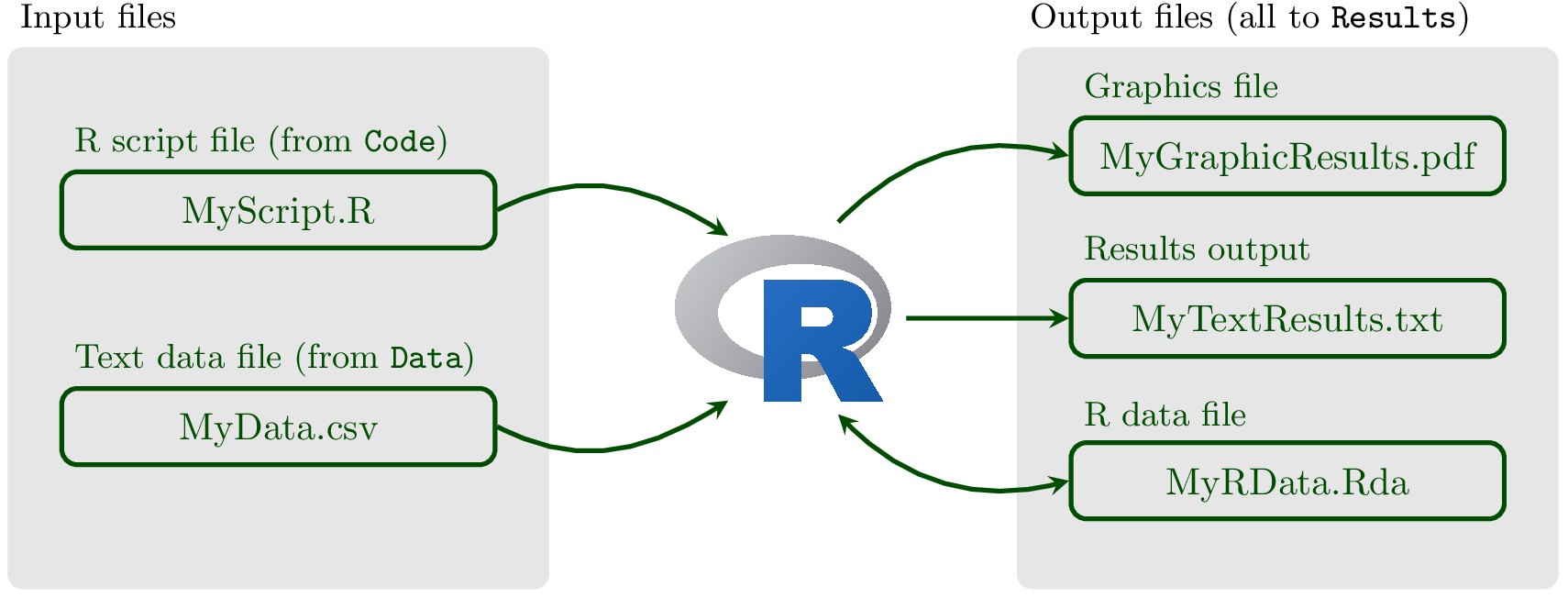
Fig. 16 Your R project. Keeping it neat and organized if the key to becoming a good R programmer.¶

Some details on each kind of file:

R script files: These are plain text files containing all the R code needed for an analysis. These should be created with a text editor, typically part of some smart code editor like vscode, or RStudio, and saved with the extension *.R. You should never use Word to save or edit these files as R can only read code from plain text files.
Text data files These are files of data in plain text format containing one or more columns of data (numbers, strings, or both). Although there are several format options, we will typically be using csv files, where the data entries are separated by commas. These are easy to create and export from Excel (if that’s what you use…).
Results output files These are a plain text files containing your results, such the the summary of output of a regression or ANOVA analysis. Typically, you will output your results in a table format where the columns are separated by commas (csv) or tabs (tab-delimited).
Graphics files R can export graphics in a wide range of formats. This can be done automatically from R code and we will look at this later but you can also select a graphics window (e.g., in RStudio) and click File $\triangleright$ Save as....
Rdata files You can save any data loaded or created in R, including outputs of statistical analyses and other things, into a singleRdata file. These are not plain text and can only be read by R, but can hold all the data from an analysis in a single handy location. We will not use these much in this course.

So let’s build your R analysis project structure.

Do the following:

★ Create a sensibly-named directory (e.g., MyRCoursework, week3, etc, depnding on which course you are on) in an appropriate location on your computer. If you are using a college Windows computer, you may need to create it in your H: drive. Avoid including spaces in your file or directory names, as this will often create problems when you share your file or directory with somebody else. Many software programs do not handle spaces in file/directory names well. Use underscores instead of spaces. For example, instead of My R Coursework, use My_R_Coursework or MyRCoursework.

★ Create subdirectories within this directory called code, data, and results. Remember, commands in all programming languages are case-sensitive when it comes to reading directory path names, so code is not the same as Code!

You can create directories using dir.create()within R (or if on Mac/Linux, with the usual mkdir from the bash terminal):

dir.create("MyRCoursework")
dir.create("MyRCoursework/code")
dir.create("MyRCoursework/data")    
dir.create("MyRCoursework/results")    

The R Workspace and Working Directory¶

R has a “workspace” – a current working environment that includes any user-defined data structures objects (vectors, matrices, data frames, lists) as well as other objects (e.g., functions). At the end of an R session, the user can save an image of the current workspace that is automatically reloaded the next time R is started. Your workspace is saved in your “Working Directory”, which has to be set manually.

So before we go any further, let’s get sort out where your R “Working Directory” should be and how you should set it. R has a default location where it assumes your working directory is.

In UNIX/Linux, it is whichever directory you are in when you launch R.
In Mac, it is /User/YourUserName or similar.
In Windows, it is C:/Windows/system32or similar.

To see where your current working directory is, at the R command prompt, type:

getwd()

This tells you what the current working directory is.

Now, set the working directory to be MrRCourseworkcode. For example, if you created MrRCourseworkdirectly in your H:\, the you would use:

setwd("H:/MrRCourseworkcode")

dir() #check what’s in the current working directory

On your own computer, you can also change R’s default to a particular working directory where you would like to start (easily done in RStudio):

In Linux, you can do this by editing the Rprofile.sitesite with sudo gedit /etc/R/Rprofile.site. In that file, you would add your start-up parameters between the lines

.First <- function() cat("\n Welcome to R!\n\n")

and

`.Last <- function() cat("\n   Goodbye! \n\n")`.

Between these two lines, insert: setwd("/home/YourName/YourDirectoryPath")

In Windows and Macs, you can find the Rprofile.sitefile by searching for it. On Windows, it should be at C:\Program Files\R\R-x.x.x\etc directory, where x.x.x is your R version.
If you are using RStudio, you can change the default working directory through the RStudio “Options” dialog.

Importing and Exporting Data¶

We are now ready to see how to import and export data in R, typically the first step of your analysis. The best option is to have your data in a comma separated value ( csv) text file or in a tab separated text file. Then, you can use the function read.csv(or read.table) to import your data. Now, lets get some data into your Datadirectory.

★ Go to the TheMulQuaBio git repository and navigate to the data directory.

★ Download and copy the file trees.csv into your own data directory.

Alternatively, of you may download the whole repository to your computer and then grab the file from the place where you downloaded it.

Now, import the data:

MyData <- read.csv("../data/trees.csv")

ls(pattern = "My*") # Check that MyData has appeared

'MyData'
'MyDF'
'MyList'
'MyMat'
'MyVar'

Your output may be somewhat different, depending on what what variables and other objects have been created in your R Workspace during the current R session. But the main thing is, you should be able to see a MyData in the list of objects printed.

Tip

You can list only objects with a particular name pattern by using the pattern option of ls(). It works by using regular expressions, which you were introduced through the grep command in the UNIX chapter. We will delve deeper into regular expressions in the Python II Chapter.

Note that the resulting MyData object in your workspace is a R dataframe:

class(MyData)

'data.frame'

Relative paths¶

Note the UNIX-like path to the file we used in the read.csv() command above (using forward slashes; Windows uses back slashes).

The ../ in read.csv("../data/trees.csv") above signifies a “relative” path. That is, you are asking R to load data that lies in a different directory (folder) relative your current location (in this case, you are in your Codedirectory). In other, more technical words, ../data/trees.txtpoints to a file named trees.txtlocated in the “parent” of the current directory.

What is an absolute path? — one that specifies the whole path on your computer, say from C:\”upwards” on Windows, /Users/ upwards on Mac, and /home/ upwards on Linux. Absolute paths are specific to each computer, so should be avoided. So to import data and export results, your script should not use absolute paths. Also, AVOID putting a setwd()command at the start of your R script, because setting the working directory requires an absolute directory path, which will differ across computers, platforms, and users. Let the end users set the working directory on their machine themselves.

Using relative paths in in your R scripts and code will make your code computer-independent and easier for others to use your code. The relative path way should always be the way you load data in your analyses scripts — it will guarantee that your analysis works on every computer, not just your own or college computer.

Tip

If you are using a computer from elsewhere in the EU, Excel may use a comma (e.g., $\pi=3,1416$) instead of a decimal point ($\pi=3.1416$). In this case, csvfiles may use a semi-colon to separate columns and you can use the alternative function read.csv2() to read them into the R workspace.

head(MyData) # Have a quick look at the data frame

A data.frame: 6 × 3
	Species	Distance.m	Angle.degrees
	<chr>	<dbl>	<dbl>
1	Populus tremula	31.66583	41.28264
2	Quercus robur	45.98499	44.53592
3	Ginkgo biloba	31.24177	25.14626
4	Fraxinus excelsior	34.61667	23.33613
5	Betula pendula	45.46617	38.34913
6	Betula pendula	48.79550	33.59231

You can also have a more detailed look at the data you imported:

str(MyData) # Note the data types of the three columns

'data.frame':	120 obs. of  3 variables:
 $ Species      : chr  "Populus tremula" "Quercus robur" "Ginkgo biloba" "Fraxinus excelsior" ...
 $ Distance.m   : num  31.7 46 31.2 34.6 45.5 ...
 $ Angle.degrees: num  41.3 44.5 25.1 23.3 38.3 ...

MyData <- read.csv("../data/trees.csv", header = F) # Import ignoring headers

head(MyData)

A data.frame: 6 × 3
	V1	V2	V3
	<chr>	<chr>	<chr>
1	Species	Distance.m	Angle.degrees
2	Populus tremula	31.6658337740228	41.2826361937914
3	Quercus robur	45.984992608428	44.5359166583512
4	Ginkgo biloba	31.2417666241527	25.1462585572153
5	Fraxinus excelsior	34.6166691975668	23.336126555223
6	Betula pendula	45.4661654261872	38.3491299510933

Or you can load data using the more general read.table function:

MyData <- read.table("../data/trees.csv", sep = ',', header = TRUE) #another way

With read.table you need to specify whether there is a header row that needs to be imported as such.

head(MyData)

A data.frame: 6 × 3
	Species	Distance.m	Angle.degrees
	<chr>	<dbl>	<dbl>
1	Populus tremula	31.66583	41.28264
2	Quercus robur	45.98499	44.53592
3	Ginkgo biloba	31.24177	25.14626
4	Fraxinus excelsior	34.61667	23.33613
5	Betula pendula	45.46617	38.34913
6	Betula pendula	48.79550	33.59231

MyData <- read.csv("../data/trees.csv", skip = 5) # skip first 5 lines

Writing to and saving files¶

You can also save your data frames using write.table or write.csv:

write.csv(MyData, "../results/MyData.csv")

dir("../results/") # Check if it worked

'LV_model.pdf'
'MyData.csv'
'MyFirst-ggplot2-Figure.pdf'
'MyResults.Rout'
'Pred_Prey_Overlay.pdf'
'QMEENet.svg'
'TreeHeight.csv'

write.table(MyData[1,], file = "../results/MyData.csv",append=TRUE) # append

Warning message in write.table(MyData[1, ], file = "../results/MyData.csv", append = TRUE):
“appending column names to file”

You get a warning with here because R thinks it is strange that you are appending headers to a file that already has headers!

write.csv(MyData, "../results/MyData.csv", row.names=TRUE) # write row names

write.table(MyData, "../results/MyData.csv", col.names=FALSE) # ignore col names

Writing R code¶

Typing in commands interactively in the R console is good for starters, but you will want to switch to putting your sequence of commands into a script file, and then ask R to run those commands.

Open a new text file, call it basic_io.R, and save it to your codedirectory.
Write the above input-output commands in it:

# A simple script to illustrate R input-output.  
# Run line by line and check inputs outputs to understand what is happening  

MyData <- read.csv("../data/trees.csv", header = TRUE) # import with headers

write.csv(MyData, "../results/MyData.csv") #write it out as a new file

write.table(MyData[1,], file = "../results/MyData.csv",append=TRUE) # Append to it

write.csv(MyData, "../results/MyData.csv", row.names=TRUE) # write row names

write.table(MyData, "../results/MyData.csv", col.names=FALSE) # ignore column names

Now place the cursor on the first line of code in the script file and run it by pressing the appropriate keyboard shortcut (e.g., PC: ctrl+R, Mac: command+enter, Linux: ctrl+enter are the usual shortcuts for doing this).
Check after every line that you are getting the expected result.

Note

Why no shebang in your first R script? Because we are learning R here mainly for writing scripts for data analysis & visualization, and relatively simple numerical calculations & modelling/simulation tasks. Read this and this for some more technical advice about R scripts.

Running R code¶

But even writing to a script file and running the code line-by-line or block-by-block is not your ultimate goal. What you would really like to do is to just run your full analysis and output all the results. There are two main approaches for running R script/code.

Using `source`¶

You can run all the contents of a *.Rscript file from the R command line by using source().

★ Try sourcing basic_io.R (you will need to make sure you have setwd to your code directory):

source("basic_io.R")

Warning message in write.table(MyData[1, ], file = "../results/MyData.csv", append = TRUE):
“appending column names to file”

That has run OK, warning and all.

If you get errors, read and then try to fix them. The most common problem is likely to be that you have not setwd() to the code directory.

Alternatively, you can run the script from wherever (e.g., data directory) by adding the directory path to the script file name, if the script file is not in your working directory and you don’t want to change your working directory. For example, you will need source("../code/control.R if your working directory is data and not code (using a relative path).

Do not put a source()command inside the script file you are sourcing, as it is then trying to run itself again and again and that’s just cruel!*

Tip

The command source()has a chdirargument whose default value is FALSE. When set to TRUE, it will change the working directory to the directory of the file being sourced.

Also, if you have sourceed a script successfully, you will see no output on in R console/terminal unless there was an error or warning, or if you explicitly asked for something to be printed. So it can be useful to add a line at the end of the script saying something like print("Script complete!").

Using `Rscript`¶

You can also run R script from the UNIX/Linux terminal by calling Rscript. That is, while you have to be inside an R session to use the source command to run a script, you can run a R script directly from the UNIX/Linux terminal by calling Rscript.

This allows you to easily automate execution of your R scripts (e.g., by writing a bash script) and integrate R into a bigger computing pipeline/workflow by calling it through other tools or languages (e.g., see the Python Chapter II).

If you are on Linux, try using Rscript to run basic_io.R:

Exit from the R console using ctrl+D, or open a new bash terminal
cd to the location of basic_io.R (e.g., week3/code)
Then run the script using Rscript basic_io.R

Also, please have a look at man Rscript in a bash terminal.

Running R in batch mode¶

In addition to Rscript, there is another way to run you R script without opening the R console. In Mac or Linux, you can do so by typing:

R CMD BATCH MyCode.R MyResults.Rout

This will create an MyResults.Routfile containing all the output. On Microsoft Windows, it’s more complicated — change the path to R.exeand output file as needed:

"C:\Program Files\R\R-4.x.x\bin\R.exe" CMD BATCH -vanilla -slave "C:\PathToMyResults\Results\MyCode.R"

Here, replace 4.x.x with the R version you have.

Control flow tools¶

In R, you can write “if-then”, and “else” statements, and “for” and “while” loops like any programming language to give you finer control over your program’s “control flow”. Such statements are useful to include in functions and scripts because you may only want to do certain calculations or other tasks, under certain conditions (e.g., if the dataset is from a particular year, do something different).

Let’s look at some examples of these control flow tools in R.

★ Type each of the following blocks of code in a script file called control_flow.R and save it in your code directory. then run each block separately by sending or pasting into the R console.

`if` statements¶

a <- TRUE
if (a == TRUE) {
    print ("a is TRUE")
} else {
    print ("a is FALSE")
}

[1] "a is TRUE"

Note that using if (a) instead of if (a == TRUE) will also achieve the same result, because a is a Boolean variable. Compare with Python conditionals.

In general, it is arguably a good idea to make explicit the if condition though.

You can also write an if statement on a single line:

z <- runif(1) ## Generate a uniformly distributed random number
if (z <= 0.5) {print ("Less than a half")}

But code readability is important, so avoid squeezing control flow blocks like this into a single line.

Tip

Please indent your code for readability, even if its not strictly necessary (unlike Python). Indentation helps you see the flow of the logic, rather than flattened version, which is hard for you and anybody else to read. For example, the following code block is so much much readable than the one above:

z <- runif(1)
if (z <= 0.5) {
    print ("Less than a half")
   }

`for` loops¶

Loops are really useful to repeat a task over some range of input values.

The following code “loops” over a range of numbers, squaring each, and then printing the result:

for (i in 1:10) {
    j <- i * i
    print(paste(i, " squared is", j ))
}

[1] "1  squared is 1"
[1] "2  squared is 4"
[1] "3  squared is 9"
[1] "4  squared is 16"
[1] "5  squared is 25"
[1] "6  squared is 36"
[1] "7  squared is 49"
[1] "8  squared is 64"
[1] "9  squared is 81"
[1] "10  squared is 100"

What exactly is going on in the piece of code above? What are i and j? Let’s break it down:

Firstly The 1:10 part simply generates a sequence, as you learned previously:

1:10

1
2
3
4
5
6
7
8
9
10

This is the same as using seq(10) (try substituting this instead of 1:10 in the above block of code).

Then, j is a temporary variable that stores the value of the number (the other temporary variable, i) in that iteration of the loop.

Note

Using the : operator or the seq() function pre-generates the sequence and stores it in memory, so is less efficient that Python’s range function, which generates numbers in a sequence on a “need-to” basis.

You can also loop over a vector of strings:

for(species in c('Heliodoxa rubinoides', 
                 'Boissonneaua jardini', 
                 'Sula nebouxii')) {
      print(paste('The species is', species))
}

[1] "The species is Heliodoxa rubinoides"
[1] "The species is Boissonneaua jardini"
[1] "The species is Sula nebouxii"

These is a random assortment of birds!

And here’s a for loop using apre-existing vector:

v1 <- c("a","bc","def")
for (i in v1) {
    print(i)
}

[1] "a"
[1] "bc"
[1] "def"

`while` loops¶

If you want to perform an operation till some condition is met, use a while loop:

i <- 0
while (i < 10) {
    i <- i+1
    print(i^2)
}

[1] 1
[1] 4
[1] 9
[1] 16
[1] 25
[1] 36
[1] 49
[1] 64
[1] 81
[1] 100

★ Now test control_flow.R. That is, run the script file using source (and Rscript if on Linux).

If you get errors, read them carefully and fix them (this is going to be your mantra henceforth!).

Some more control flow tools¶

Let’s look at some more control tools that are less commonly used, but can be useful in certain scenarios.

`break`ing out of loops¶

Often it is useful (or necessary) to break out of a loop when some condition is met. Use break (like in pretty much any other programming language, like Python) in situations when you cannot set a target number of iterations and would like to stop the loop execultion once some condition is met (as you would with a while loop).

Try this (type into break.R and save in code):

i <- 0 #Initialize i
    while (i < Inf) {
        if (i == 10) {
            break 
        } else { # Break out of the while loop!  
            cat("i equals " , i , " \n")
            i <- i + 1 # Update i
    }
}

i equals  0  
i equals  1  
i equals  2  
i equals  3  
i equals  4  
i equals  5  
i equals  6  
i equals  7  
i equals  8  
i equals  9  

Using `next`¶

You can also skip to next iteration of a loop. Both next and break can be used within other loops ( while, for). Try this (type into next.R and save in code):

for (i in 1:10) {
  if ((i %% 2) == 0) # check if the number is odd
    next # pass to next iteration of loop 
  print(i)
}

[1] 1
[1] 3
[1] 5
[1] 7
[1] 9

This code checks if a number is odd using the “modulo” operation and prints it if it is.

Writing R Functions¶

A function is a block of re-useable code that takes an input, does something with it (or to it!), and returns the result. Like any other programming language, R lets you write your own functions. All the “commands” that you have been using, such as ls(), mean(), c(), etc are basically functions. You will want to write your own function for every scenario where a particular task or set of analysis steps need to be performed again and again.
The syntax for R functions is quite simple, with each function accepting “arguments” and “returning” a value.

Your first R function¶

★ Type the following into a script file called boilerplate.Rand save it in your code directory:

# A boilerplate R script

MyFunction <- function(Arg1, Arg2) {
  
  # Statements involving Arg1, Arg2:
  print(paste("Argument", as.character(Arg1), "is a", class(Arg1))) # print Arg1's type
  print(paste("Argument", as.character(Arg2), "is a", class(Arg2))) # print Arg2's type
    
  return (c(Arg1, Arg2)) #this is optional, but very useful
}

MyFunction(1,2) #test the function
MyFunction("Riki","Tiki") #A different test

Note the curly brackets – these are necessary for R to know where the specification of the function starts and ends. Also, note the indentation. Not necessary (unlike Python), but recommended to make the code more readable.

Now enter the R console and source the script:

source("boilerplate.R")

[1] "Argument 1 is a numeric"
[1] "Argument 2 is a numeric"
[1] "Argument Riki is a character"
[1] "Argument Tiki is a character"

This will run the script, and also save your function MyFunction as an object into your workspace (try ls(), and you will see MyFunction appear in the list of objects):

ls(pattern = "MyFun*")

'MyFunction'

Again, you output may be a bit different as you have been different things in your R workspace/session than I have. What matters is that you see MyFunction in the list of objects above.

Now try:

class(MyFunction)

'function'

So, yes, MyFunctionis a function objec, just as it would be in Python.

Functions with conditionals¶

Here are some examples of functions with conditionals:

# Checks if an integer is even
is.even <- function(n = 2) {
  if (n %% 2 == 0) {
    return(paste(n,'is even!'))
  } else {
  return(paste(n,'is odd!'))
  }
}

is.even(6)

'6 is even!'

# Checks if a number is a power of 2
is.power2 <- function(n = 2) {
  if (log2(n) %% 1==0) {
    return(paste(n, 'is a power of 2!'))
  } else {
  return(paste(n,'is not a power of 2!'))
    }
}

is.power2(4)

'4 is a power of 2!'

# Checks if a number is prime
is.prime <- function(n) {
  if (n==0) {
    return(paste(n,'is a zero!'))
  } else if (n==1) {
    return(paste(n,'is just a unit!'))
  }
    
  ints <- 2:(n-1)
  
  if (all(n%%ints!=0)) {
    return(paste(n,'is a prime!'))
  } else {
  return(paste(n,'is a composite!'))
    }
}

is.prime(3)

'3 is a prime!'

★ Run the three blocks of code in R one at a time and make sure you understand what each function is doing and how. Save all three blocks to a single script file called R_conditionals.R in your code directory, and make sure it runs using source and Rscript (in the Linux/Ubuntu terminal) .

An example utility function¶

Now let’s write a script containing a more useful function:

★ In your text editor type the following in a file called TreeHeight.R, and save it in your codedirectory:

# This function calculates heights of trees given distance of each tree 
# from its base and angle to its top, using  the trigonometric formula 
#
# height = distance * tan(radians)
#
# ARGUMENTS
# degrees:   The angle of elevation of tree
# distance:  The distance from base of tree (e.g., meters)
#
# OUTPUT
# The heights of the tree, same units as "distance"

TreeHeight <- function(degrees, distance) {
    radians <- degrees * pi / 180
    height <- distance * tan(radians)
    print(paste("Tree height is:", height))
  
    return (height)
}

TreeHeight(37, 40)

Run TreeHeight.R’s two blocks (the TreeHeight function, and the call to the function, TreeHeight(37, 40)) by pasting them sequentially into the R console. Try and understand what each line is doing.
Now test the whole TreeHeight.R script at one go using source and/or Rscript (in Linux/Ubuntu).

Practicals¶

Tree heights¶

Modify the script TreeHeight.R so that it does the following:

Loads trees.csv and calculates tree heights for all trees in the data. Note that the distances have been measured in meters. (Hint: use relative paths)).

Creates a csv output file called TreeHts.csv in resultsthat contains the calculated tree heights along with the original data in the following format (only first two rows and headers shown):

"Species","Distance.m","Angle.degrees","Tree.Height.m"
"Populus tremula",31.6658337740228,41.2826361937914,27.8021161438536
"Quercus robur",45.984992608428,44.5359166583512,45.2460250644405

This script should work using either source or Rscript in Linux / UNIX.

Groupwork Practical on Tree Heights¶

The goal of this practical is to make the TreeHeight.R script more general, so that it could be used for other datasets, not just trees.csv.

Guidelines:

Write another R script called get_TreeHeight.R that takes a csv file name from the command line (e.g., get_TreeHeight.R Trees.csv) and outputs the result to a file just like TreeHeight.Rabove, but this time includes the input file name in the output file name as InputFileName_treeheights.csv. Note that you will have to strip the .csvor whatever the extension is from the filename, and also ../ etc., if you are using relative paths. (Hint: Command-line parameters are accessible within the R running environment via commandArgs() — so help(commandArgs) might be your starting point.)
Write a Unix shell script called run_get_TreeHeight.sh that tests get_TreeHeight.R. Include trees.csvas your example file. Note that sourcewill not work in this case as it does not allow scripts with arguments to be run; you will have to use Rscriptinstead.

Groupwork Practical on Tree Heights 2¶

Assuming you have already worked through Python Chapter I, write a Python version of get_TreeHeight.R (call it get_TreeHeight.py). Include a test of this script into run_get_TreeHeight.sh.

Vectorization¶

R is relatively slow at cycling through a data structure such as a dataframe or matrix (e.g., by using a for loop) because it is a high-level, interpreted computer language.

That is, when you execute a command in R, it needs to “read” and interpret the necessary code from scratch every single time the command is called. On the other hand, compiled languages like C know exactly what the flow of the program is because the code is pre-interpreted and ready to go before execution (i.e., the code is “compiled”).

For example, when you assign a new variable in R:

a <- 1.0
class(a)

'numeric'

R automatically figures out that 1.0 is an floating point number, and finds a place in the system memory for it with a registered as a “pointer” to it.

In contrast, in C, for example, you would have to do so manually by giving a an address and space in memory:

float a
a = 1

Vectorization is an approach where you directly apply compiled, optimized code to run an operation on a vector, matrix, or an higher-dimensional data structure (like an R array), instead of performing the operation element-wise (each row or column element one at a time) on the data structure.

Apart from computational efficiency vectorization makes writing code more concise, easy to read, and less error prone.

Let’s try an example that illustrates this point.

★ Type (save in Code) as Vectorize1.R the following script, and run it (it sums all elements of a matrix):

M <- matrix(runif(1000000),1000,1000)

SumAllElements <- function(M) {
  Dimensions <- dim(M)
  Tot <- 0
  for (i in 1:Dimensions[1]) {
    for (j in 1:Dimensions[2]) {
      Tot <- Tot + M[i,j]
    }
  }
  return (Tot)
}
 
print("Using loops, the time taken is:")
print(system.time(SumAllElements(M)))

print("Using the in-built vectorized function, the time taken is:")
print(system.time(sum(M)))

[1] "Using loops, the time taken is:"
   user  system elapsed 
   0.08    0.00    0.08 
[1] "Using the in-built vectorized function, the time taken is:"
   user  system elapsed 
  0.001   0.000   0.001 

Note the system.time R function: it calculates how much time your code takes. This time will vary with every run, and every computer that this code is run on (so your times will be a bit different than what I got).

Both SumAllElements() and sum() approaches are correct, and will give you the right answer. However, the inbuilt function sum() is about 100 times faster than the other, because it uses vectorization, avoiding the amount of looping that SumAllElements() uses.

In effect, of course, the computer still has to run loops. However, this running of the loops is encapsulated in a pre-complied program that R calls. These programs are written in more primitive (and therefore, faster) languages like Fortran and C. For example sum is actually written in C if you look under the hood.

In R, even if you should try to avoid loops, in practice, it is often much easier to throw in a for loop, and then “optimize” the code to avoid the loop if the running time is not satisfactory. Therefore, it is still essential that you to become familiar with loops and looping as you learned in the sections above.

Pre-allocation¶

And if you are using loops, one operation that is slow in R (and somewhat slow in all languages) is memory allocation for a particular variable that will change during looping (e.g., a variable that is a dataframe). So writing a for loop that resizes a vector repeatedly makes R re-allocate memory repeatedly, which makes it slow. Try this:

NoPreallocFun <- function(x) {
    a <- vector() # empty vector
    for (i in 1:x) {
        a <- c(a, i) # concatenate
        print(a)
        print(object.size(a))
    }
}

system.time(NoPreallocFun(10))

[1] 1
56 bytes
[1] 1 2
56 bytes
[1] 1 2 3
64 bytes
[1] 1 2 3 4
64 bytes
[1] 1 2 3 4 5
80 bytes
[1] 1 2 3 4 5 6
80 bytes
[1] 1 2 3 4 5 6 7
80 bytes
[1] 1 2 3 4 5 6 7 8
80 bytes
[1] 1 2 3 4 5 6 7 8 9
96 bytes
 [1]  1  2  3  4  5  6  7  8  9 10
96 bytes

   user  system elapsed 
  0.011   0.000   0.011 

Here, in each repetition of the for loop, you can see that R has to re-size the vector and re-allocate (more) memory. It has to find the vector in memory, create a new vector that will fit more data, copy the old data over, insert the new data, and erase the old vector. This can get very slow as vectors get big.

On the other hand, if you “pre-allocate” a vector that fits all the values, R doesn’t have to re-allocate memory each iteration. Here’s how you’d do that for the above case:

PreallocFun <- function(x) {
    a <- rep(NA, x) # pre-allocated vector
    for (i in 1:x) {
        a[i] <- i # assign
        print(a)
        print(object.size(a))
    }
}

system.time(PreallocFun(10))

 [1]  1 NA NA NA NA NA NA NA NA NA
96 bytes
 [1]  1  2 NA NA NA NA NA NA NA NA
96 bytes
 [1]  1  2  3 NA NA NA NA NA NA NA
96 bytes
 [1]  1  2  3  4 NA NA NA NA NA NA
96 bytes
 [1]  1  2  3  4  5 NA NA NA NA NA
96 bytes
 [1]  1  2  3  4  5  6 NA NA NA NA
96 bytes
 [1]  1  2  3  4  5  6  7 NA NA NA
96 bytes
 [1]  1  2  3  4  5  6  7  8 NA NA
96 bytes
 [1]  1  2  3  4  5  6  7  8  9 NA
96 bytes
 [1]  1  2  3  4  5  6  7  8  9 10
96 bytes

   user  system elapsed 
  0.006   0.000   0.005 

★ Write the above two blocks of code into a script called preallocate.R. You can’t really see the difference in timing here using system.time() because the vector is really small (just 10 elements), and the print() commands take up most of the time. To really see the difference in efficiency between the two functions, increase the iterations in your script from 10 to 1000, and suppress the print commands. Make this modification to your script. The modified script should print just the outputs of the two system.time() calls.

Fortunately, R has several functions that can operate on entire vectors and matrices without requiring looping (Vectorization). That is, vectorizing a computer program means you write it such that as many operations as possible are applied to whole data structure (vectors, matrices, dataframes, lists, etc) at one go, instead of its individual elements.

You will learn about some important R functions that allow vectorization in the following sections.

The `*apply` family of functions¶

There are a family of functions called *apply in R that vectorize your code for you. These functions are described in the help files (e.g. ?apply).

For example, apply can be used when you want to apply a function to the rows or columns of a matrix (and higher-dimensional analogues – remember arrays!). This is not generally advisable for data frames as it will first need to coerce the data frame to a matrix first.

Let us try using applying the same function to rows/colums of a matrix using apply.

★ Type the following in a script file called apply1.R, save it to your Code directory, and run it:

## Build a random matrix
M <- matrix(rnorm(100), 10, 10)

## Take the mean of each row
RowMeans <- apply(M, 1, mean)
print (RowMeans)

 [1]  0.36031151  0.04436538  0.22147423  0.20493801  0.16210725  0.04860134
 [7]  0.41767343 -0.30198204  0.17624371 -0.12782576

## Now the variance
RowVars <- apply(M, 1, var)
print (RowVars)

 [1] 0.8054302 0.5757168 0.3312622 0.4285847 0.9819718 0.9878042 0.6637336
 [8] 0.8063847 0.4404945 1.3378551

## By column
ColMeans <- apply(M, 2, mean)
print (ColMeans)

 [1]  0.225188540 -0.005593872  0.070236505  0.540658047  0.207704657
 [6] -0.039456952 -0.308016915 -0.052139549 -0.017257915  0.584584511

That was using apply on some of R’s inbuilt functions. You can use apply to define your own functions. Let’s try it.

★ Type the following in a script file called apply2.R, save it to your Code directory, and run it:

SomeOperation <- function(v) { # (What does this function do?)
  if (sum(v) > 0) { #note that sum(v) is a single (scalar) value
    return (v * 100)
  } else { 
  return (v)
    }
}

M <- matrix(rnorm(100), 10, 10)
print (apply(M, 1, SomeOperation))

            [,1]        [,2]       [,3]        [,4]       [,5]      [,6]
 [1,] -234.39455   31.662431  0.7233882 -0.94436410 -1.4572646 -20.07141
 [2,]  180.15974   83.582155  0.3644622  1.19740008 -0.3927685 -98.37526
 [3,]   16.28549  143.665254  0.3018886 -1.06216206 -2.3448302 224.24758
 [4,]  -28.24259   -6.671888  0.4672368  0.63864658  0.4280011 -86.77100
 [5,]  237.42028  148.139235  1.2226815  0.04541425 -0.3694419 -17.01924
 [6,]   67.62704   14.332068 -0.3192625 -1.51307536 -1.8384410 -15.53040
 [7,]  107.61127   53.433940 -1.8648914 -0.10926190 -1.3273339  87.13306
 [8,]   39.42281 -101.533491  0.1049022 -0.58231320 -0.1164919  80.88842
 [9,]   85.01566  177.863389 -2.0382452 -0.06725732  0.6842362 -39.28277
[10,]   79.61237   67.051809  0.3626656  0.40823357 -1.1903160  27.77324
             [,7]       [,8]        [,9]       [,10]
 [1,] -0.90120256  18.385375  0.04279667    3.696104
 [2,] -0.48180877  74.636647 -0.97886275  147.825300
 [3,] -0.65661220   9.031228  0.69408658   57.520424
 [4,] -0.49917243 -94.532163 -0.41680049  128.188540
 [5,]  0.07449752 163.795799 -0.57998084  -22.925171
 [6,] -0.31465171 -82.500457  0.09081916 -106.962944
 [7,]  0.76765184   9.721098 -1.81725821   42.298713
 [8,]  1.99041007  73.372002 -0.29073832  133.662999
 [9,]  0.93981016 -28.824632  1.31045316  129.069991
[10,] -1.45123295 126.623928 -1.11812957   69.367728

Thus, the function SomeOperation takes as input v. Then if the sum of v is greater than zero, it multiplies that value by 100. So if v has positive and negative numbers, and the sum comes out to be positive, only then does it multiply all the values in v by 100 and return them.

There are many other methods: lapply, sapply, eapply, etc. Each is best for a given data type. For example, lapply abd sapply are designed for R lists. Have a look at this Stackoveflow thread for some guidelines.

A vectorization example¶

Let’s try an example of vectorization involving lapply and sapply. Both of these apply a function to each element of a list, but the former returns a list, while the latter returns a vector.

We will also see how sampling random numbers works in the process of trying out this example.

★ Type the following blocks of code into a single script called sample.R and save in code.

First some functions:

######### Functions ##########

## A function to take a sample of size n from a population "popn" and return its mean
myexperiment <- function(popn,n) {
    pop_sample <- sample(popn, n, replace = FALSE)
    return(mean(pop_sample))
}

## Calculate means using a FOR loop on a vector without preallocation:
loopy_sample1 <- function(popn, n, num) {
    result1 <- vector() #Initialize empty vector of size 1 
    for(i in 1:num) {
        result1 <- c(result1, myexperiment(popn, n))
    }
    return(result1)
}

## To run "num" iterations of the experiment using a FOR loop on a vector with preallocation:
loopy_sample2 <- function(popn, n, num) {
    result2 <- vector(,num) #Preallocate expected size
    for(i in 1:num) {
        result2[i] <- myexperiment(popn, n)
    }
    return(result2)
}

## To run "num" iterations of the experiment using a FOR loop on a list with preallocation:
loopy_sample3 <- function(popn, n, num) {
    result3 <- vector("list", num) #Preallocate expected size
    for(i in 1:num) {
        result3[[i]] <- myexperiment(popn, n)
    }
    return(result3)
}


## To run "num" iterations of the experiment using vectorization with lapply:
lapply_sample <- function(popn, n, num) {
    result4 <- lapply(1:num, function(i) myexperiment(popn, n))
    return(result4)
}

## To run "num" iterations of the experiment using vectorization with sapply:
sapply_sample <- function(popn, n, num) {
    result5 <- sapply(1:num, function(i) myexperiment(popn, n))
    return(result5)
}

Think carefully about what each of these functions does.

Now let’s generate a population. To get the same result every time, let’s set seed (you might want to review this section).

set.seed(12345)
popn <- rnorm(10000) # Generate the population
hist(popn)

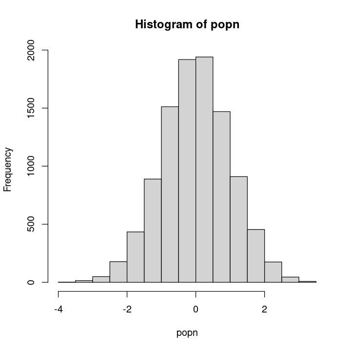
And run and time the different functions:

n <- 100 # sample size for each experiment
num <- 10000 # Number of times to rerun the experiment

print("Using loops without preallocation on a vector took:" )
print(system.time(loopy_sample1(popn, n, num)))

print("Using loops with preallocation on a vector took:" )
print(system.time(loopy_sample2(popn, n, num)))

print("Using loops with preallocation on a list took:" )
print(system.time(loopy_sample3(popn, n, num)))

print("Using the vectorized sapply function (on a list) took:" )
print(system.time(sapply_sample(popn, n, num)))

print("Using the vectorized lapply function (on a list) took:" )
print(system.time(lapply_sample(popn, n, num)))

[1] "Using loops without preallocation on a vector took:"
   user  system elapsed 
  0.596   0.000   0.651 
[1] "Using loops with preallocation on a vector took:"
   user  system elapsed 
  0.378   0.000   0.384 
[1] "Using loops with preallocation on a list took:"
   user  system elapsed 
  0.347   0.000   0.347 
[1] "Using the vectorized sapply function (on a list) took:"
   user  system elapsed 
  0.299   0.000   0.300 
[1] "Using the vectorized lapply function (on a list) took:"
   user  system elapsed 
  0.340   0.000   0.342 

Note that these times will be different on your computer because they depend on the computer’s hardware and software (especially, the operating system), as well as what other processes are running.

★ Run sample.R using source and/or Rscript and make sure it works.

Rerun the script a few times, first by fixing the n and num parameters, and then also by varying them. Compare the times you get from these repeated runs of the script and think about which approach is the most efficient and why. Clearly, the loopy, witout pre-allocation apporach is usually (but not always) going to be bad, while the others are pretty comparable.

The `tapply` function¶

Let’s look at tapply, which is particularly useful because it allows you to apply a function to subsets of a vector in a dataframe, with the subsets defined by some other vector in the same dataframe, usually a factor (this could be useful for pound hill data analysis that’s coming up, for example).

This makes it a bit of a different member of the *apply family. Try this:

x <- 1:20 # a vector
x

1
2
3
4
5
6
7
8
9
10
11
12
13
14
15
16
17
18
19
20

Now create a factor type variable (of the same length) defining groups:

y <- factor(rep(letters[1:5], each = 4)) 
y

a
a
a
a
b
b
b
b
c
c
c
c
d
d
d
d
e
e
e
e

Levels:

'a'
'b'
'c'
'd'
'e'

Now add up the values in x within each subgroup defined by y:

tapply(x, y, sum)

a: 10
b: 26
c: 42
d: 58
e: 74

Using `by`¶

You can also do something similar to tapply with the by function, i.e., apply a function to a dataframe using some factor to define the subsets. Try this:

First import some data:

attach(iris)
iris

The following objects are masked from iris (pos = 3):

    Petal.Length, Petal.Width, Sepal.Length, Sepal.Width, Species

A data.frame: 150 × 5
Sepal.Length	Sepal.Width	Petal.Length	Petal.Width	Species
<dbl>	<dbl>	<dbl>	<dbl>	<fct>
5.1	3.5	1.4	0.2	setosa
4.9	3.0	1.4	0.2	setosa
4.7	3.2	1.3	0.2	setosa
4.6	3.1	1.5	0.2	setosa
5.0	3.6	1.4	0.2	setosa
5.4	3.9	1.7	0.4	setosa
4.6	3.4	1.4	0.3	setosa
5.0	3.4	1.5	0.2	setosa
4.4	2.9	1.4	0.2	setosa
4.9	3.1	1.5	0.1	setosa
5.4	3.7	1.5	0.2	setosa
4.8	3.4	1.6	0.2	setosa
4.8	3.0	1.4	0.1	setosa
4.3	3.0	1.1	0.1	setosa
5.8	4.0	1.2	0.2	setosa
5.7	4.4	1.5	0.4	setosa
5.4	3.9	1.3	0.4	setosa
5.1	3.5	1.4	0.3	setosa
5.7	3.8	1.7	0.3	setosa
5.1	3.8	1.5	0.3	setosa
5.4	3.4	1.7	0.2	setosa
5.1	3.7	1.5	0.4	setosa
4.6	3.6	1.0	0.2	setosa
5.1	3.3	1.7	0.5	setosa
4.8	3.4	1.9	0.2	setosa
5.0	3.0	1.6	0.2	setosa
5.0	3.4	1.6	0.4	setosa
5.2	3.5	1.5	0.2	setosa
5.2	3.4	1.4	0.2	setosa
4.7	3.2	1.6	0.2	setosa
⋮	⋮	⋮	⋮	⋮
6.9	3.2	5.7	2.3	virginica
5.6	2.8	4.9	2.0	virginica
7.7	2.8	6.7	2.0	virginica
6.3	2.7	4.9	1.8	virginica
6.7	3.3	5.7	2.1	virginica
7.2	3.2	6.0	1.8	virginica
6.2	2.8	4.8	1.8	virginica
6.1	3.0	4.9	1.8	virginica
6.4	2.8	5.6	2.1	virginica
7.2	3.0	5.8	1.6	virginica
7.4	2.8	6.1	1.9	virginica
7.9	3.8	6.4	2.0	virginica
6.4	2.8	5.6	2.2	virginica
6.3	2.8	5.1	1.5	virginica
6.1	2.6	5.6	1.4	virginica
7.7	3.0	6.1	2.3	virginica
6.3	3.4	5.6	2.4	virginica
6.4	3.1	5.5	1.8	virginica
6.0	3.0	4.8	1.8	virginica
6.9	3.1	5.4	2.1	virginica
6.7	3.1	5.6	2.4	virginica
6.9	3.1	5.1	2.3	virginica
5.8	2.7	5.1	1.9	virginica
6.8	3.2	5.9	2.3	virginica
6.7	3.3	5.7	2.5	virginica
6.7	3.0	5.2	2.3	virginica
6.3	2.5	5.0	1.9	virginica
6.5	3.0	5.2	2.0	virginica
6.2	3.4	5.4	2.3	virginica
5.9	3.0	5.1	1.8	virginica

Now run the colMeans function (it is better for dataframes than just mean) on multiple columns:

by(iris[,1:2], iris$Species, colMeans)

iris$Species: setosa
Sepal.Length  Sepal.Width 
       5.006        3.428 
------------------------------------------------------------ 
iris$Species: versicolor
Sepal.Length  Sepal.Width 
       5.936        2.770 
------------------------------------------------------------ 
iris$Species: virginica
Sepal.Length  Sepal.Width 
       6.588        2.974 

by(iris[,1:2], iris$Petal.Width, colMeans)

iris$Petal.Width: 0.1
Sepal.Length  Sepal.Width 
        4.82         3.36 
------------------------------------------------------------ 
iris$Petal.Width: 0.2
Sepal.Length  Sepal.Width 
    4.972414     3.379310 
------------------------------------------------------------ 
iris$Petal.Width: 0.3
Sepal.Length  Sepal.Width 
    4.971429     3.328571 
------------------------------------------------------------ 
iris$Petal.Width: 0.4
Sepal.Length  Sepal.Width 
    5.300000     3.785714 
------------------------------------------------------------ 
iris$Petal.Width: 0.5
Sepal.Length  Sepal.Width 
         5.1          3.3 
------------------------------------------------------------ 
iris$Petal.Width: 0.6
Sepal.Length  Sepal.Width 
         5.0          3.5 
------------------------------------------------------------ 
iris$Petal.Width: 1
Sepal.Length  Sepal.Width 
    5.414286     2.371429 
------------------------------------------------------------ 
iris$Petal.Width: 1.1
Sepal.Length  Sepal.Width 
    5.400000     2.466667 
------------------------------------------------------------ 
iris$Petal.Width: 1.2
Sepal.Length  Sepal.Width 
        5.78         2.74 
------------------------------------------------------------ 
iris$Petal.Width: 1.3
Sepal.Length  Sepal.Width 
    5.884615     2.746154 
------------------------------------------------------------ 
iris$Petal.Width: 1.4
Sepal.Length  Sepal.Width 
      6.3250       2.9125 
------------------------------------------------------------ 
iris$Petal.Width: 1.5
Sepal.Length  Sepal.Width 
    6.183333     2.816667 
------------------------------------------------------------ 
iris$Petal.Width: 1.6
Sepal.Length  Sepal.Width 
       6.375        3.100 
------------------------------------------------------------ 
iris$Petal.Width: 1.7
Sepal.Length  Sepal.Width 
        5.80         2.75 
------------------------------------------------------------ 
iris$Petal.Width: 1.8
Sepal.Length  Sepal.Width 
    6.400000     2.941667 
------------------------------------------------------------ 
iris$Petal.Width: 1.9
Sepal.Length  Sepal.Width 
        6.34         2.68 
------------------------------------------------------------ 
iris$Petal.Width: 2
Sepal.Length  Sepal.Width 
    6.650000     3.016667 
------------------------------------------------------------ 
iris$Petal.Width: 2.1
Sepal.Length  Sepal.Width 
    6.916667     3.033333 
------------------------------------------------------------ 
iris$Petal.Width: 2.2
Sepal.Length  Sepal.Width 
    6.866667     3.200000 
------------------------------------------------------------ 
iris$Petal.Width: 2.3
Sepal.Length  Sepal.Width 
      6.9125       3.0875 
------------------------------------------------------------ 
iris$Petal.Width: 2.4
Sepal.Length  Sepal.Width 
    6.266667     3.100000 
------------------------------------------------------------ 
iris$Petal.Width: 2.5
Sepal.Length  Sepal.Width 
    6.733333     3.400000 

Using `replicate`¶

The replicate function is useful to avoid a loop for function that typically involves random number generation (more on this below). For example:

replicate(10, runif(5))

A matrix: 5 × 10 of type dbl
0.05779543	0.79875145	0.48499984	0.86907132	0.1283642	0.0009810759	0.6536405	0.8683811	0.8454915	0.8783501
0.45615105	0.57098740	0.23039036	0.30154024	0.2747319	0.2428520240	0.9098087	0.6079378	0.6468676	0.7984627
0.56282049	0.04613426	0.62504519	0.04747557	0.7813629	0.8418969549	0.4024599	0.6946761	0.6771371	0.2471511
0.47753585	0.69846828	0.46303515	0.25758230	0.2651486	0.1114152884	0.1513297	0.3396491	0.8450003	0.3601890
0.63433648	0.40640785	0.07475354	0.04436429	0.0915491	0.2450728263	0.4717760	0.4990844	0.7130802	0.9336190

That is, you just generated 10 sets (columns) of 5 uniformly-distributed random numbers (a 10 $\times$ 5 matrix).

Note

The actual numbers you get will be different from the ones you see here unless you set the random number seed as we learned above.

Using `plyr` and `ddply`¶

The plyr package combines the functionality of the *apply family, into a few handy functions. Look up the web page.

In particular, ddply is very useful, because for each subset of a data frame, it applies a function and then combines results into another data frame. In other words, “ddply” means: take a data frame, split it up, do something to it, and return a data frame. Look up this and this for examples. There you will also see a comparison of speed of ddply vs by at the latter web page; ddply is actually slower than other vectorized methods, as it trades-off compactness of use for some of the speed of vectorization! Indeed, overall functions in plyr can be slow if you are working with very large datasets that involve a lot of subsetting (analyses by many groups or grouping variables).

The base *apply functions remain useful and worth knowing even if you do get into plyr or better still, dplyr, which we will see in the Data chapter.

Practicals¶

A vectorization challenge¶

The Ricker model is a classic discrete population model which was introduced in 1954 by Ricker to model recruitment of stock in fisheries. It gives the expected number (or density) $N_{t+1}$ of individuals in generation $t + 1$ as a function of the number of individuals in the previous generation $t$:

\[ N_{t+1}= N_t e^{r\left(1-\frac{N_t}{k}\right)} \]

Here $r$ is intrinsic growth rate and $k$ as the carrying capacity of the environment. Try this script (call it Ricker.R and save it to code) that runs it:

Ricker <- function(N0=1, r=1, K=10, generations=50)
{
  # Runs a simulation of the Ricker model
  # Returns a vector of length generations
  
  N <- rep(NA, generations)    # Creates a vector of NA
  
  N[1] <- N0
  for (t in 2:generations)
  {
    N[t] <- N[t-1] * exp(r*(1.0-(N[t-1]/K)))
  }
  return (N)
}

plot(Ricker(generations=10), type="l")

Now open and run the script Vectorize2.R (available on the TheMulQuaBio repository). This is the stochastic Ricker model (compare with the above script to see where the stochasticity (random error) enters). Now modify the script to complete the exercise given. Your goal is to come up with a solution better than mine!

Errors and Debugging¶

As we learned in Python Chapter I, dealing with errors is a fundamental programming task that never really goes away!

Unit testing¶

We will not cover unit testing here, which we did in Python Chapter I). Unit testing in R is equally recommended if you are going to develop complex code and packages.

Tip

A very convenient tool for R unit testing is testthat.

In addition, you can use other “defensive programming” methods in R to keep an eye on errors that might arise in special circumstances in an complex program. A good option for this is to convert warnings to errors using the stopifnot(). This is a bit like try (which we will cover below, and we also covered in Python Chapter I).

Debugging¶

Once you have found an error, you need to debug it. Assuming you have an idea about where (or the general area) in your code the error is, a simple way to debug is to use the browser() function.

The browser() function allows you to insert a breakpoint in your script (where the running of the script is stopped) and then step through your code. Place it within your script at the point you want to examine local variables (e.g. inside a for loop).

Let’s look at an example usage of browser().

★ Type the following in a script file called browse.R and save in code:

Exponential <- function(N0 = 1, r = 1, generations = 10) {
  # Runs a simulation of exponential growth
  # Returns a vector of length generations
  
  N <- rep(NA, generations)    # Creates a vector of NA
  
  N[1] <- N0
  for (t in 2:generations) {
    N[t] <- N[t-1] * exp(r)
    browser()
  }
  return (N)
}

plot(Exponential(), type="l", main="Exponential growth")

The script will be run till the first iteration of the for loop and the console will enter the browser mode, which looks like this:

Browse[1]>

Now, you can examine the variables present at that point. Also, at the browser console, you can enter expressions as normal, or use a few particularly useful debug commands (similar to the Python debugger):

n: single-step
c: exit browser and continue
Q: exit browser and abort, return to top-level.

Tip

We will not cover advanced debugging here as we did in Python Chapter I, but look up traceback() (to find where the errors(s) are when a program crashes), and debug() (to debug a whole function).

“Catching” errors¶

Often, you don’t know if a simulation or a R function will work on a particular data or variable, or a value of a variable (can happen in many statistical functions).

Indeed, as most of you must have already experienced by now, there can be frustrating, puzzling bugs in programs that lead to mysterious errors. Often, the error and warning messages you get are un-understandable, especially in R!

Rather than having R throw you out of the code, you would rather catch the error and keep going. This can be done by using the try keyword.

Lets try try!

First, let’s write a function:

doit <- function(x) {
    temp_x <- sample(x, replace = TRUE)
    if(length(unique(temp_x)) > 30) {#only take mean if sample was sufficient
         print(paste("Mean of this sample was:", as.character(mean(temp_x))))
        } 
    else {
        stop("Couldn't calculate mean: too few unique values!")
        }
    }

This function runs a simulation that involves sampling from a synthetic population with replacement and takes its mean, but only if at least 30 unique samples are obtained. Note that we have used another keyword here: stop(). Pay close attention to sample(), and stop() in the above script (check out what they are by using R help or searching online).

Now, generate your population:

set.seed(1345) # again, to get the same result for illustration

popn <- rnorm(50)

hist(popn)

Now try running it using lapply as you did above, repeating the sampling exercise 15 times:

lapply(1:15, function(i) doit(popn))

[1] "Mean of this sample was: -0.11620822588674"
[1] "Mean of this sample was: -0.0468516755995931"
[1] "Mean of this sample was: -0.0890228211466614"
[1] "Mean of this sample was: -0.124229742255296"

Error in doit(popn): Couldn't calculate mean: too few unique values!
Traceback:

1. lapply(1:15, function(i) doit(popn))
2. FUN(X[[i]], ...)
3. doit(popn)   # at line 1 of file <text>
4. stop("Couldn't calculate mean: too few unique values!")   # at line 7 of file <text>

Your result will be different than this (you would get between 0 - 15 samples; we got 4 here). But in most cases, the script will fail because of the stop command (on line 7 of the above function) at some iteration, returning less than the requested 15 mean values, followed by an error stating that the mean could not be calculated because too few unique values were sampled.

Now try doing the same using try:

result <- lapply(1:15, function(i) try(doit(popn), FALSE))

[1] "Mean of this sample was: -0.11620822588674"
[1] "Mean of this sample was: -0.0468516755995931"
[1] "Mean of this sample was: -0.0890228211466614"
[1] "Mean of this sample was: -0.124229742255296"
Error in doit(popn) : Couldn't calculate mean: too few unique values!
[1] "Mean of this sample was: 0.0314144452816157"
[1] "Mean of this sample was: -0.233476945796405"
[1] "Mean of this sample was: -0.196681538928001"
[1] "Mean of this sample was: 0.0146969612111605"
[1] "Mean of this sample was: -0.234913159471725"
[1] "Mean of this sample was: -0.0497464588165691"
Error in doit(popn) : Couldn't calculate mean: too few unique values!
[1] "Mean of this sample was: 0.14834078393269"
[1] "Mean of this sample was: -0.271626543849156"
[1] "Mean of this sample was: -0.0661949014450445"

In this run, you again asked for the means of 15 samples, and again you (most likely) got less than that (see the above example output), but without any error! The FALSE modifier for the try command suppresses any error messages, but result will still contain them so that you can inspect them later (see below). Please don’t forget to check the help on inbuilt R commands like try.

The errors are stored in the object result:

class(result)

'list'

This is a list that stores the result of each of the 15 runs, including the ones that ran into an error. Have a look at it:

result

[[1]]
[1] "Error in doit(popn) : Couldn't calculate mean: too few unique values!\n"
attr(,"class")
[1] "try-error"
attr(,"condition")
<simpleError in doit(popn): Couldn't calculate mean: too few unique values!>

[[2]]
[1] "Mean of this sample was: -0.0639710889231533"

[[3]]
[1] "Mean of this sample was: 0.0954898884134274"

[[4]]
[1] "Error in doit(popn) : Couldn't calculate mean: too few unique values!\n"
attr(,"class")
[1] "try-error"
attr(,"condition")
<simpleError in doit(popn): Couldn't calculate mean: too few unique values!>

[[5]]
[1] "Mean of this sample was: 0.179497884968553"

[[6]]
[1] "Mean of this sample was: -0.0269560049619619"

[[7]]
[1] "Mean of this sample was: -0.0596177312603713"

[[8]]
[1] "Error in doit(popn) : Couldn't calculate mean: too few unique values!\n"
attr(,"class")
[1] "try-error"
attr(,"condition")
<simpleError in doit(popn): Couldn't calculate mean: too few unique values!>

[[9]]
[1] "Mean of this sample was: -0.169305162448064"

[[10]]
[1] "Mean of this sample was: -0.0570172067888256"

[[11]]
[1] "Mean of this sample was: 0.130501940679632"

[[12]]
[1] "Mean of this sample was: -0.0476960671278198"

[[13]]
[1] "Error in doit(popn) : Couldn't calculate mean: too few unique values!\n"
attr(,"class")
[1] "try-error"
attr(,"condition")
<simpleError in doit(popn): Couldn't calculate mean: too few unique values!>

[[14]]
[1] "Mean of this sample was: -0.0103821907230653"

[[15]]
[1] "Error in doit(popn) : Couldn't calculate mean: too few unique values!\n"
attr(,"class")
[1] "try-error"
attr(,"condition")
<simpleError in doit(popn): Couldn't calculate mean: too few unique values!>

That’s a lot output! But basically it tells you which runs ran into and error and why (no surprises here, of course!). You can also store the results “manually” by using a loop to do the same:

result <- vector("list", 15) #Preallocate/Initialize
for(i in 1:15) {
    result[[i]] <- try(doit(popn), FALSE)
    }

[1] "Mean of this sample was: 0.0690929258795289"
[1] "Mean of this sample was: -0.117793922564727"
Error in doit(popn) : Couldn't calculate mean: too few unique values!
[1] "Mean of this sample was: 0.179353333942007"
[1] "Mean of this sample was: 0.00392019401996458"
[1] "Mean of this sample was: -0.0432275201290453"
Error in doit(popn) : Couldn't calculate mean: too few unique values!
[1] "Mean of this sample was: -0.0869881356850989"
Error in doit(popn) : Couldn't calculate mean: too few unique values!
[1] "Mean of this sample was: 0.0984080957232758"
Error in doit(popn) : Couldn't calculate mean: too few unique values!
[1] "Mean of this sample was: 0.0856480925151331"
[1] "Mean of this sample was: 0.0462039547120371"
Error in doit(popn) : Couldn't calculate mean: too few unique values!
[1] "Mean of this sample was: -0.0147578826249971"

Now have a look at the new result; it will have similar content as the one you got from using lapply.

Tip

Also check out tryCatch() as an alternative to try().

★ Type the above blocks of code illustrating try into a script file called try.R and save in code. The script, when sourced, should run without errors (that is, don’t run the sampling function without try!).

Packages¶

The big strength of R is that users can easily build and share packages through cran.r-project.org.

There are R packages for practically all statistical and mathematical analysis you might conceive, so check them out before reinventing the wheel. Visit cran.r-project.org and go to packages to see a list and a brief description.

In Windows and Macs and Linux, you can install a package within R by using the install.packages()command.

For example:

install.packages(c("tidyverse"))

You can also install multiple packages by concatenating their names: install.packages(c("pack1","pack2","pack3")) (three packages in this hypothetical example)

In Ubuntu, you will have to launch a sudo Rsession to get install.packages()to work properly. Otherwise, you be forced to install the package in a non-standard location on your drive that does not require sudo privileges (nor recommended).

You can also use the RStudio GUI to install packages using your mouse and menu.

In Ubuntu, you can also use the bash terminal:

sudo apt install r-cran-tidyverse

★ Go ahead and install tidyverse if you don’t have it yet. We will be using it soon!

Building your own¶

You can combine your code, data sets and documentation to make a bona fide R package. You may wish to do this for particularly large projects that you think will be useful for others. Read the Writing R Extensions manual and see package.skeleton to get started.

The R tool set EcoDataTools and the package cheddar were written by Silwood Grad Students!

Practicals¶

Is Florida getting warmer?¶

This Practical assumes you have at least a basic understanding of correlation coefficients and p-values.

Your goal is to write an R script that will help answer the question: Is Florida getting warmer? Call this script Florida.R.

To answer the question, you need to calculate the correlation coefficients between temperature and time. However, you can’t use the standard p-value calculated for a correlation coefficient, because measurements of climatic variables in successive time-points in a time series (successive seconds, minutes, hours, months, years, etc.) are not independent. Therefore you will use a permutation analysis instead, by generating a distribution of random correlation coefficients and compare your observed coefficient with this random distribution.

Some guidelines:

Load and examine the annual temperature dataset from Key West in Florida, USA for the 20th century:

rm(list=ls())

load("../data/KeyWestAnnualMeanTemperature.RData")

ls()

'ats'

class(ats)

'data.frame'

head(ats)

A data.frame: 6 × 2
	Year	Temp
	<int>	<dbl>
1	1901	23.75000
2	1902	24.66667
3	1903	24.71667
4	1904	24.51667
5	1905	24.88333
6	1906	24.63333

plot(ats)

Then,

Compute the appropriate correlation coefficient between years and Temperature and store it (look at the help file for cor()
Repeat this calculation a sufficient number of times, each time randomly reshuffling the temperatures (i.e., randomly re-assigning temperatures to years), and recalculating the correlation coefficient (and storing it)

Tip

You can use the sample function that we learned about above to do the shuffling. Read the help file for this function and experiment with it.

Calculate what fraction of the random correlation coefficients were greater than the observed one (this is your approximate, asymptotic p-value).
Interpret and present the results: Present your results and their interpretation in a pdf document written in $\LaTeX$ (include the the document’s source code in the submission) (Keep the writeup, including any figures, to one A4 page).

Groupwork Practical: Autocorrelation in Florida weather¶

This Practical assumes you have at least a basic understanding of correlation coefficients and p-values.

Your goal is to write an R script (name it TAutoCorr.R) that will help answer the question: Are temperatures of one year significantly correlated with the next year (successive years), across years in a given location?

To answer this question, you need to calculate the correlation between (n-1) pairs of years, where $n$ is the total number of years. However, here again, you can’t use the standard p-value calculated for a correlation coefficient, because measurements of climatic variables in successive time-points in a time series (successive seconds, minutes, hours, months, years, etc.) are not independent.

The general guidelines are:

Compute the appropriate correlation coefficient between successive years and store it (look at the help file for cor()
Repeat this calculation a sufficient number of times by – randomly permuting the time series, and then recalculating the correlation coefficient for each randomly permuted sequence of annual temperatures and storing it.
Then calculate what fraction of the correlation coefficients from the previous step were greater than that from step 1 (this is your approximate p-value).
Interpret and present the results Present your results and their interpretation in a pdf document written in $\LaTeX$ (submit the the document’s source code as well).

Readings and Resources¶

Check the readings under the R directory in the TheMulQuaBio repository. Also, search online for “R tutorial”, and plenty will pop up. Choose ones that seem the most intuitive to you. * Remember, all R packages come with pdf guides/documentation!

R as a Programming language¶

There are excellent websites besides cran. In particular, check out statmethods.net and the R Wiki.
https://blog.sellorm.com/2017/12/18/learn-to-write-command-line-utilities-in-r/
https://www.r-bloggers.com/2019/11/r-scripts-as-command-line-tools/

Mathematical modelling and Stats in R¶

The Use R! series (all yellow books) by Springer are really good. In particular, consider: “A Beginner’s Guide to R”, “R by Example”, “Numerical Ecology With R”, “ggplot2” (coming up in the Visualization Chapter, “A Primer of Ecology with R”, “Nonlinear Regression with R”, and “Analysis of Phylogenetics and Evolution with R”.
For more focus on dynamical models: Soetaert & Herman. 2009 “A practical guide to ecological modelling: using R as a simulation platform”.

Debugging¶

testthat: Unit Testing for R by Hadley Wickham (also developer of the tidyverse package, including ggplot).
Notes on debugging in R by Wickham
A good overview of debugging methods in R with examples
An introduction to the Interactive Debugging Tools in R by Roger D Peng.
If you are using RStudio, see this.

Sweave and knitr, and beyond¶

There are tools built around R that allow you to write your Dissertation Report or some other document such that it can be updated automatically if embedded data analyses or R simulations / calculations change. Instead of inserting a prefabricated graph or table into the report, the master document contains the R code necessary to obtain it. When run through R, all data analysis output (tables, graphs, etc.) is created on the fly and inserted into a final document like a pdf or html. The report will then be automatically updated if data or analysis change, which allows for truly reproducible research. To learn more about these tools, check out:

Sweave and knitr and this
Quarto

TheMulQuaBio

Biological Computing in R

Contents

Biological Computing in R¶

Introduction¶

Why R?¶

Would you ever need anything other than R?¶

Installing R¶

Getting started¶

R basics¶

Useful R commands¶

Baby steps¶

Variable names and Tabbing¶

Operators¶

When things go wrong¶

Types of parentheses¶

Variable types¶

Type Conversions and Special Values¶

R Data Structures¶

Vectors¶

Matrices and arrays¶

Data frames¶

Lists¶

Matrix vs Dataframe¶

Creating and manipulating data¶

Creating sequences¶

Accessing parts of data stuctures: Indices and Indexing¶

Recycling¶

Basic vector-matrix operations¶

Strings and Pasting¶

Useful R functions¶

For manipulating strings¶

Mathematical¶

Statistical¶

Sets¶

Generating Random Numbers¶

“Seeding” random number generators¶

Your analysis workflow¶

The R Workspace and Working Directory¶

Importing and Exporting Data¶

Relative paths¶

Writing to and saving files¶

Writing R code¶

Running R code¶

Using source¶

Using Rscript¶

Running R in batch mode¶

Control flow tools¶

if statements¶

for loops¶

while loops¶

Some more control flow tools¶

breaking out of loops¶

Using next¶

Writing R Functions¶

Your first R function¶

Functions with conditionals¶

An example utility function¶

Practicals¶

Tree heights¶

Groupwork Practical on Tree Heights¶

Groupwork Practical on Tree Heights 2¶

Vectorization¶

Pre-allocation¶

The *apply family of functions¶

A vectorization example¶

The tapply function¶

Using by¶

Using replicate¶

Using plyr and ddply¶

Practicals¶

A vectorization challenge¶

Errors and Debugging¶

Unit testing¶

Debugging¶

“Catching” errors¶

Packages¶

Building your own¶

Practicals¶

Is Florida getting warmer?¶

Using `source`¶

Using `Rscript`¶

`if` statements¶

`for` loops¶

`while` loops¶

`break`ing out of loops¶

Using `next`¶

The `*apply` family of functions¶

The `tapply` function¶

Using `by`¶

Using `replicate`¶

Using `plyr` and `ddply`¶